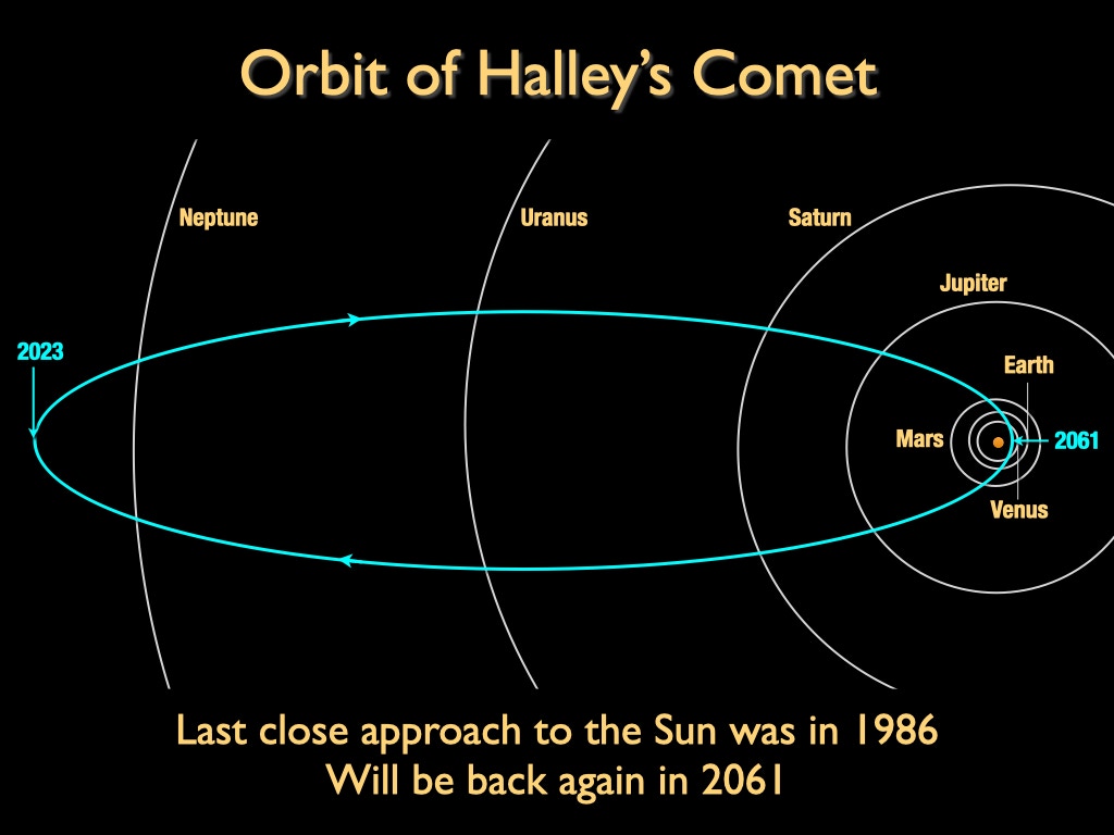
At the end of the 17th century, comets were still regarded as unpredictable, accidental phantoms streaking across the sky. Astronomer Edmond Halley decided to challenge this perception. Rather than relying on isolated observations or personal intuition, he systematically gathered and curated centuries of historical comet sighting records—a time-series dataset spanning space and time. Upon analyzing these records, Halley noticed that the orbital parameters of the comets appearing in 1531, 1607, and 1682 were strikingly similar. He put forward a bold hypothesis: these were not three separate comets, but a single celestial body returning on a regular schedule. He calculated its orbital period to be roughly 76 years and made a grand prediction based on it: the comet would appear once again in 1758.

From Celestial Cycles to Statistical Thought: The Origins of Sequence Modeling#

In 1758, the comet arrived right on schedule, brilliantly validating Halley’s prediction. In a system governed by deterministic laws (such as universal gravitation), once we successfully distill those underlying rules from data, we can make pinpoint long-term forecasts. However, when we step back from the starry sky down to human society, finding such a simple, eternal “divine formula” is practically impossible.

From the swings of financial markets and the fluctuations of commodity prices to the continuous flow of everyday human language, the real-world states of these sequences are driven by countless minute, dynamic, and even unobservable factors, brimming with uncertainty. Yet our human desire to peer into the future feels innate, and time-series analysis—as a specialized subfield of statistics—was born precisely to tackle this class of problems. It focuses on analyzing data points indexed in temporal order, typically relying on assumptions such as stationarity to perform statistical modeling and inference.

Throughout the 20th century, the field of time-series analysis was dominated by two primary schools of thought. One was the Box-Jenkins methodology centered on ARMA models, which excelled at modeling relatively stationary sequences and left a profound imprint on economics. The other comprised state-space models represented by the Kalman filter, which achieved milestone successes in signal processing fields requiring dynamic tracking and control.

Despite the differing theoretical emphases and application domains of these two schools, they shared two core conceptual pillars that are deeply relevant to our theme, ultimately serving as the bedrock of modern RNNs:

1. Time Invariance

In statistics, this concept typically corresponds to the stationarity assumption, which posits that a process’s statistical properties (such as mean and variance) do not change over time. Interpreted from a deeper conceptual standpoint, stationarity implies that the underlying “rules” driving data generation remain constant.

This resonates profoundly with the translational symmetry we encountered in Convolutional Neural Networks (CNNs): both assume the existence of a universal pattern or rule that applies across different temporal (or spatial) locations in the data. This principle of universality is the fundamental motivation behind parameter sharing in neural networks.

2. The Markov Assumption

Among Markov assumptions, the first-order assumption is the most concise and influential. Its precise formulation states that the state at any given moment depends solely on the state at the immediately preceding moment, and has no direct dependence on earlier history.

When our objective is to make effective predictions, the implications shift—if a model is to maintain robust predictive power while adhering to the Markov assumption, its internal representation of the “current state” must be sufficiently rich and comprehensive.

Thus, we can view the Markov assumption from another angle: it requires the model to learn how to efficiently “absorb” critical information from a lengthy history into its representation of the present state.

These two ideas—that rules are invariant across time, and that the future depends only on an continuously updated current state—jointly gave birth to an elegant and powerful dynamic evolution framework: the Recurrent Neural Network (RNN).

Its core architecture can be expressed in an abstract functional form:

This equation encapsulates the operational logic of an RNN: the new state h_t at the next moment (also known as the hidden state) is jointly determined by the old state h_{t-1} from the previous moment and the new external input x_t received at the current moment; subsequently, the output y_t at the current moment is generated directly from this new state h_t.

It is worth emphasizing that, unlike CNNs which introduced specialized neural network operations like convolution and pooling, the distinguishing feature of early RNNs was not the introduction of a novel type of operation—the inner workings of their core computation unit f(\cdot) still relied on familiar combinations of linear layers and activation functions, or basic arithmetic.

The true innovation of the RNN lies in its recurrent structure: reusing the exact same set of computational weights across the temporal dimension, thereby forging a bridge between the present and the past.

Recurrent Neural Networks: The Challenge of Memory and the Gating Revolution#

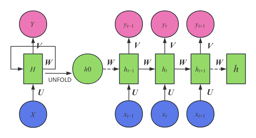
The core idea of a recurrent neural network is to maintain a running memory of historical information via a hidden state vector passed recursively across time steps.

At each time step t, the network performs two operations: first, it takes the current input x_t and the previous hidden state h_{t-1}, generating a new hidden state h_t via shared transformations; second, it produces the current output y_t based on this new hidden state.

In its original and simplest formulation, the exact computations are:

In this architecture, the weight matrices W, U, V and bias terms b_h, b_y remain constant across all time steps (time invariance), while h_t depends directly only on h_{t-1} (the Markov assumption). Theoretically, it can process sequences of arbitrary length and capture complex dynamic patterns.

However, this seemingly elegant recurrent structure harbors a fatal Achilles’ heel during training, making it notoriously difficult to learn long-term dependencies within sequences.

Its training algorithm—Backpropagation Through Time (BPTT)—requires gradient signals from the loss function to be propagated backward along the chain of unrolled time steps. According to the chain rule, this process inevitably involves repeated multiplications by the exact same weight matrix W.

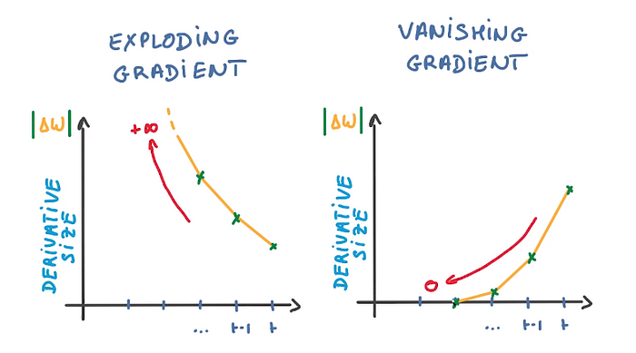
This gives rise to severe numerical instabilities: if the spectral radius of matrix W (i.e., the absolute value of its largest eigenvalue) is less than 1, gradient signals decay exponentially during backpropagation, eventually vanishing to zero—a phenomenon known as the vanishing gradient problem; conversely, if the spectral radius is greater than 1, gradients grow exponentially, causing numerical overflow—known as the exploding gradient problem.

Vanishing gradients prevent the model from receiving effective learning signals from the distant past, while exploding gradients instantly crash the training process. Consequently, vanilla RNNs suffer from a built-in “short-term memory” bias, rendering them inadequate for tasks that demand genuine long-term recollection.

To conquer this hurdle and endow neural networks with reliable long-term memory, the Long Short-Term Memory (LSTM) network was engineered.

The revolutionary innovation of LSTM lies in its decision not to “fix” the single hidden state, but rather to introduce an independent Cell State acting as a dedicated information “conveyer belt.” Alongside this, it incorporates a sophisticated Gating Mechanism that actively and meticulously manages this information flow, much like a skilled engineer.

Next, let us break down the internal information flow within an LSTM unit step by step to see how it achieves long-term memory through coordinated “valves.”

The Five-Step Memory Management Process of LSTM#

1. Step One: Receiving Inputs

Before performing any calculations, an LSTM unit first ingests three crucial sources of information: the previous short-term memory (the hidden state h_{t-1}), the external input at the current moment (x_t), and the previous long-term memory (referred to as the cell state C_{t-1}).

All subsequent gating calculations revolve around these three information streams to decide how to update memories and generate outputs.

It is worth noting that while LSTM introduces the novel concept of a “cell state,” its essence remains part of the RNN hidden state. We can view LSTM as a refined design that splits the originally monolithic hidden state into two coordinated components: “long-term memory” (cell state) and “short-term memory” (hidden state)—entirely consistent with the general definition of an RNN.

2. Step Two: The Forget Gate — Deciding What to Discard

First, the LSTM must evaluate which pieces of information inherited from the past long-term memory C_{t-1} have become obsolete and should be discarded.

This is handled by the forget gate, a Sigmoid layer that receives the short-term memory h_{t-1} and external input x_t, outputting a number between 0 and 1 for every number in C_{t-1}. Here, 1 means “keep entirely,” while 0 means “forget completely.”

3. Step Three: The Input Gate — Deciding What to Store

Next, the network needs to determine what new information should be stored in the long-term cell state.

This process unfolds in two parts: first, an input gate (another Sigmoid layer receiving h_{t-1} and x_t) decides which values to update; second, a \tanh layer creates a vector of candidate new memories based on the same inputs.

4. Step Four: Updating the Cell State — Executing Memory Revision

Now, the LSTM is ready to update the cell state.

It multiplies the old long-term memory C_{t-1} by the output of the forget gate, dropping the information it decided to forget. Then, it adds the product of the input gate’s output and the candidate memory vector—incorporating the new information.

Finally, it sums these two results to produce the brand-new cell state C_t. This addition-centric update step is paramount: it establishes an additive gradient “highway” that allows gradients to flow smoothly backward during backpropagation, dramatically alleviating the vanishing gradient problem.

5. Step Five: The Output Gate — Deciding What to Output

Finally, the network determines its current output h_t (which serves as both the step’s final output and the short-term memory for the next time step) based on the updated long-term memory C_t.

The output gate passes through a Sigmoid layer to decide which parts of the cell state will be outputted, and then passes the cell state through a \tanh layer (squashing values between -1 and 1) before multiplying them together to yield the final output h_t.

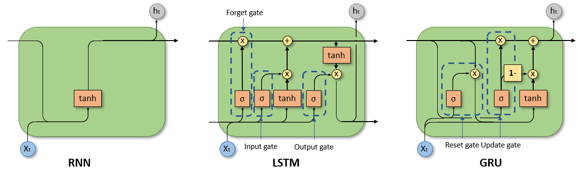
It is worth mentioning that while the aforementioned combination of Sigmoid and \tanh represents the classic LSTM design, it is not set in stone. Subsequent research has explored substituting alternative activation functions like ReLU to optimize model dynamics. More fundamental than the choice of activation function is the architectural concept of “gating” pioneered by LSTM itself.

Following the resounding success of LSTMs, researchers discovered that their internal structure could be streamlined, leading to the Gated Recurrent Unit (GRU) as one of the most popular variants.

The GRU merges LSTM’s forget and input gates into a single “update gate” and consolidates the cell state and hidden state into one. This leaves GRU with fewer parameters and higher computational efficiency while matching LSTM performance across many tasks, making it a widely favored choice.

At this point, by introducing sophisticated gating mechanisms, researchers had transformed a passive update structure prone to information loss into an active management system capable of selectively sustaining long-term context—empowering neural network models for the very first time to reliably process long sequences.

The next challenge naturally shifted from the unit level to the architectural level: how to combine these powerful units into end-to-end models capable of tackling more complex tasks?

Beyond Recurrence: The Rise of the Seq2Seq Architecture and Attention Mechanisms#

In truth, prior to 2014, LSTMs had not truly exploded in popularity within the natural language processing domain. This was because the input and output sequences of standard LSTM models were tightly coupled; their mode of operation resembled simultaneous translation—hearing a word meant immediately translating it, requiring the input and output rhythms (lengths) to align closely.

For complex tasks like intelligent question-answering where input and output sequence lengths frequently differ, researchers needed a new architectural paradigm.

The turning point arrived with a model named Seq2Seq (Sequence-to-Sequence) in 2014. As illustrated below, rather than modifying the internal structure of LSTM/GRU units, it designed a two-stage workflow where an Encoder and a Decoder decoupled the “reading” and “generating” processes:

1. Encoder

Operating like a deeply focused reader, the encoder digests the entire input sequence and “compresses” it into a fixed-length vector known as the Context Vector (e.g., [0.13, -0.54, 0.88, \ldots]).

This vector encapsulates all the information in the sequence—spanning semantics, grammar, and emotional tone.

2. Decoder

Operating like a creator working from an outline, the decoder takes the context vector generated by the encoder as its “creative blueprint” (its initial hidden state) and generates the output sequence token by token (of arbitrary length) until the work is complete.

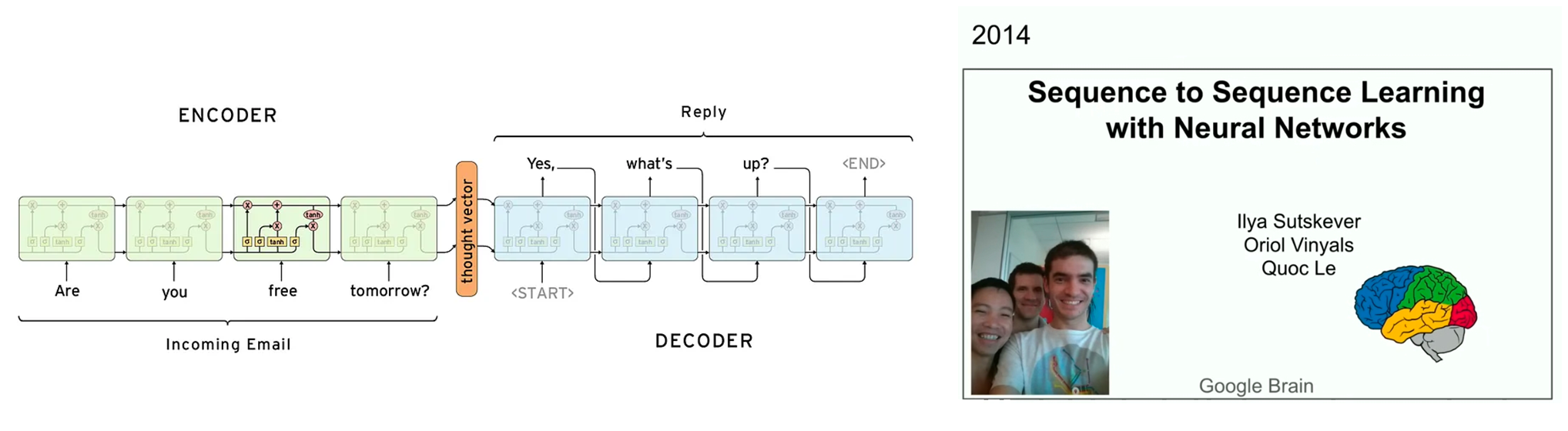
This “encode first, decode second” Seq2Seq architecture achieved remarkable success. Notably, its primary inventor was none of other than Ilya Sutskever—later co-founder and former chief scientist of OpenAI, and the core mastermind behind the development of the GPT series.

The irony of this history is that while Seq2Seq laid the foundation for subsequent language models, ChatGPT’s ultimate form required discarding Seq2Seq’s core design entirely. What lay behind this pivot?

The answer is that when confronted with excessively long input sequences, this architecture suffered from an inherent, “fatal” flaw—the Information Bottleneck.

Intuitively speaking, it required the encoder to cram the contents of a thousand-page ancient manuscript onto a tiny palm-sized index card, hand it to the decoder, and expect it to understand the entire book from that slip of paper. Yet the capacity of that index card (the context vector) is strictly finite; a vast amount of crucial detail is bound to be lost. Thus, no matter how clever the encoder might be, the quality and accuracy of its output remained severely constrained.

Consequently, researchers began to reflect: forcing all information to pass through a single hidden state seemed excessively harsh.

Instead of making the decoder rely entirely on this heavily compressed context vector, why not empower it to “look back” and dynamically extract the most relevant information directly from different parts of the input sequence whenever it generates each output token?

This insight birthed the core component of the next-generation sequence model—the Attention Mechanism.

Attention in RNNs#

Specifically, its workflow can be broken down into the following steps:

1. Forming a Query: At each decoding step, the decoder generates a “query” or “cue” based on its current hidden state, representing the exact information it needs most at that moment.

2. Computing Scores: The model compares this “query” against the information at every position in the input sequence, computing a “relevance score” for each position.

3. Weight Normalization: These scores are normalized (typically using a Softmax function) into a set of weights known as Attention Weights. This weight distribution clearly indicates how much “attention” various parts of the input sequence deserve at the current decoding step.

4. Weighted Summation: Finally, the model computes a weighted sum of the input sequence parts based on these attention weights, generating a custom context vector dynamically tailored for the current step to guide the final output.

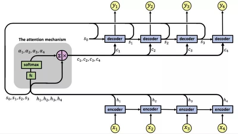
How, precisely, is this “relevance score” calculated? There are two mainstream approaches, reflecting different design trade-offs:

• Bahdanau Attention (Additive Attention): This approach introduces a dedicated, small feed-forward neural network to learn the alignment between the “query” (decoder hidden state) and the “keys” (encoder hidden states). Because it models alignment via an independent network layer, its expressive power is higher, but it incurs higher computational overhead.

• Luong Attention (Multiplicative Attention): This approach relies on direct dot products (or bilinear variants) to compute similarity. It is computationally hyper-efficient as it introduces virtually no new learnable parameters, but its effectiveness depends on whether the vector spaces of the “query” and “keys” naturally capture semantic similarity.

This attention mechanism freed models from having to “rote-memorize” the entire input sequence, allowing them to dynamically extract the most relevant pieces of information based on the task at hand.

In machine translation, for example, generating a verb might prompt the model to look at the subject and object in the source sentence, whereas generating an adjective instantly shifts attention to the modified noun. The combination of RNNs + Attention quickly became the mainstream paradigm for sequence processing.

Undoubtedly, attention mechanisms offered a powerful tool bridging arbitrary sequence positions.

This naturally leads to a subversive question: if attention alone is powerful enough to capture long-range dependencies, is the step-by-step, marching-in-order recurrent computation performed by RNNs to maintain sequence order still necessary? Might it actually be the bottleneck holding back parallel computing capabilities?

GeoAI — What Are We Predicting About Spatiotemporal Data?#

Conventionally, this section might have presented readers with a neat catalog of “classic applications” of RNNs in GeoAI. In reality, however, defining a “classic application” is trickier than it seems.

Traffic flow prediction certainly involves geographic space and its attributes, yet that domain has long formed a self-contained ecosystem within computer science time-series forecasting. Moreover, the elegance of model designs is typically rooted in the specific data properties they are built to address.

Without building a foundational worldview of spatiotemporal data, models like Transformers and Diffusion entering the scene in subsequent chapters risk becoming exercises in pure technical jargon.

Therefore, this section is not meant to tell readers how to model, but rather to plant a seed of contemplation regarding “space and time.”

As subsequent chapters unfold, this seed may gradually sprout. When you encounter a new GeoAI model, you will naturally ask: How does it reflect spatial heterogeneity? How does it handle spatiotemporal dependencies?

Before reading this section, you might ponder: What on earth are we predicting when it comes to spatiotemporal data? Answering that requires us to examine the intersections of historical and modern thought.

From “Ancient” to “Modern”: The Immutable Properties of Time#

As noted in the opening of this chapter, prior to the rise of deep learning, time-series forecasting relied heavily on statistical methods whose core mission was extracting the intrinsic regularities of data.

Although these methods may look “archaic” today, they laid down the core mental paradigms we use to understand and build time-series models today.

1. Decomposition: Finding Patterns Amid Complex Fluctuations#

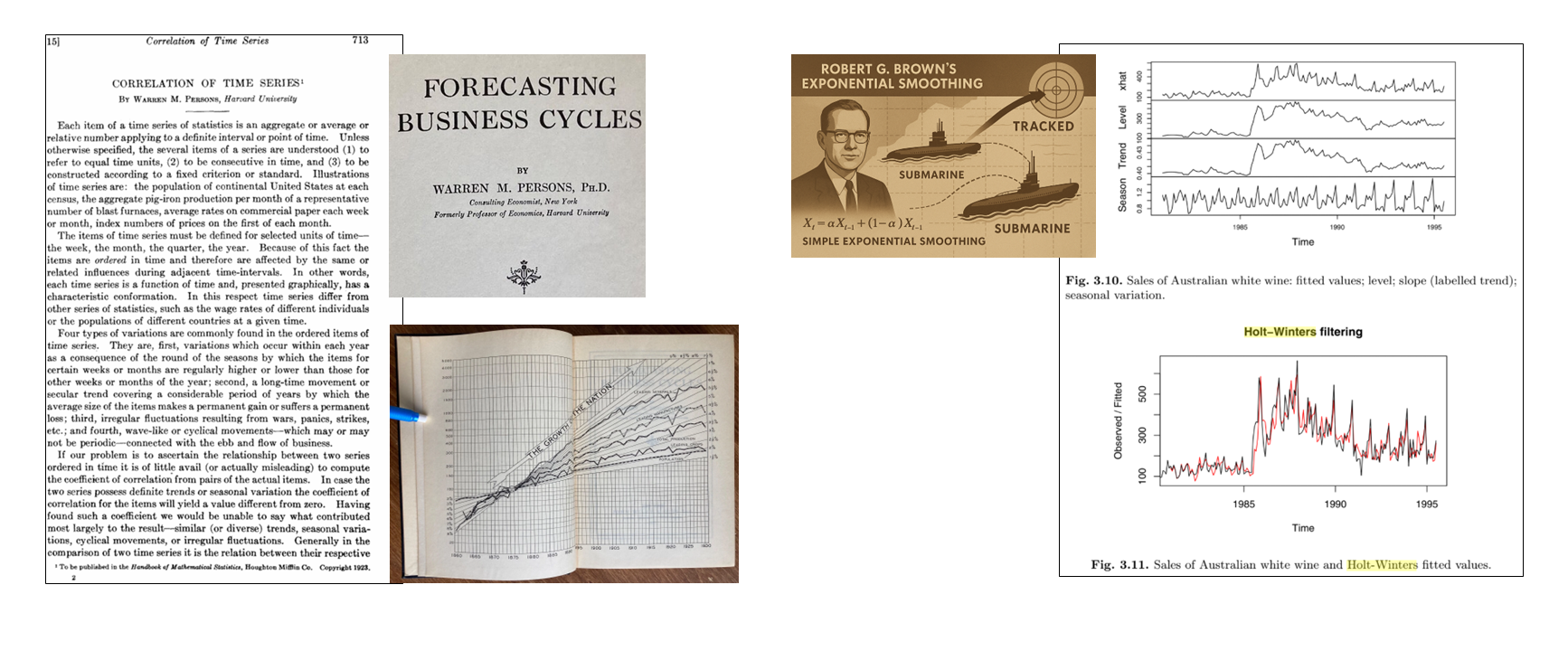
Decomposition was among the earliest attempts to break down time series into “relatively stable” components—namely Trend (T), Seasonality (S), Cyclicality (C), and Residual/Randomness (I).

Originating from the work of early 20th-century economists and business statisticians, these methods sought to identify regularities more clearly by stripping away components across different temporal scales when facing complex economic volatility.

This mindset carried over into deep learning, evolving into concepts like “multi-scale modeling” and “structured representations.”

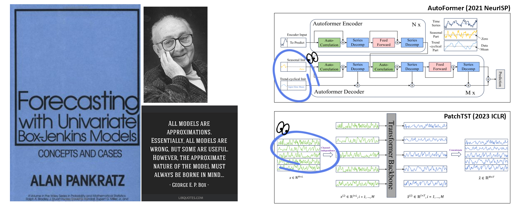
N-BEATS (2019) is a direct descendant of this philosophy: it uses deep fully-connected networks to learn a set of basis function coefficients and fits trends and seasonalities via linear combinations, sparking widespread attention with its stellar performance on the M4 forecasting benchmark.

Autoformer (2021) went a step further by internalizing the decomposition principle as a differentiable structural component within the network, allowing the model to automatically decompose and reconstruct signals during processing.

2. Exponential Smoothing: Temporal Decay and Memory#

Exponential Smoothing emphasizes “temporal decay and memory”—recent observations carry more information about the future than older ones and should therefore be assigned larger weights that decay exponentially into the past.

Evolving in the latter half of World War II, these methods satisfied the urgent demand for rapid, automated forecasting of military supplies. A prime example is the Holt-Winters triple exponential smoothing method proposed in 1960, which combined exponential smoothing with trend and seasonality to form a hybrid framework blending “memory” and “decomposition.”

conceptually, this shares a striking resemblance with LSTM gating mechanisms: both decide whether information should be retained or forgotten. There is nothing new under the sun; even today’s cutting-edge models often echo the shadows of historical methods.

3. ARIMA: The Culmination of Classical Time-Series Forecasting#

The Autoregressive Integrated Moving Average (ARIMA) model fused the ideas of decomposition and exponential smoothing. Proposed by George Box and Gwilym Jenkins in the 1970s, it stands as a milestone in time-series forecasting.

Let us unpack the letters in ARIMA:

• AR (AutoRegressive): The future is a continuation of the past; historical data harbors predictive clues about the future, so past values (lagged terms) are used as features.

Mathematically expressed as:

• MA (Moving Average): Modeling should account for the shock effects of historical prediction “errors,” hence past forecast residuals are leveraged to correct current predictions.

• I (Integrated): Converting non-stationary series into stationary ones by subtracting the previous value from the current value (differencing).

Thus, starting from the temporal properties of data, ARIMA integrated the three core pillars of time-series modeling: autocorrelation (acknowledging temporal dependencies), trend and seasonality (decomposing temporal patterns), and exponential decay (recency bias).

Many contemporary deep learning time-series frameworks largely inherit and re-express these ideas—clever innovations often amount to taking “first principles” proven effective by history and re-expressing them more efficiently using modern tools (whether CNNs, RNNs, Transformers, or architectures yet to be born).

The World Is an Open, Complex System#

Returning to our overarching question: What are we predicting regarding spatiotemporal data?

Astute readers may have noticed that the classical methods discussed above effectively construct an endogenous, closed system for the data, where forecasts represent extrapolations purely driven by internal autocorrelation and trend inertia.

However, the real world is an open, complex system frequently perturbed by “external forces”: taking traffic flow prediction as an example, a sudden rainstorm, a traffic accident, or the letting out of a concert can instantly shatter the system’s “inertia.”

Moreover, identical events trigger vastly different consequences depending on location:

• A heavy rainstorm might paralyze traffic in the city center while leaving suburban roads merely slick.
• A main arterial accident generates a vastly larger spatial extent and duration of congestion than an accident on a secondary side street.

This highlights a core principle in geospatial analysis: Spatial Non-stationarity—the relationships among variables shift across geographic space.

It is precisely this profound awareness of spatiotemporal dependencies—characterized by “here versus there” and “now versus then”—that sets GeoAI apart from traditional time-series forecasting. Let us observe how this “spatiotemporal mindset” manifested across models of different eras.

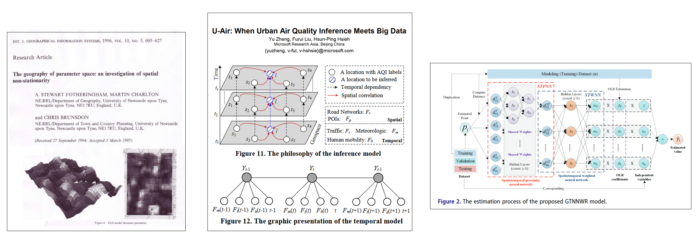
Viewed through this lens, spatiotemporal prediction is fundamentally relationship modeling within a complex system: integrating historical system states (temporal dimension), external driving factors (weather, events), and neighborhood spatial influences to approximate the system state at the “current moment” and extrapolate into the future.

Under the lens of GeoAI, deep learning models are leveraged to automatically learn hidden patterns and relationships during spatiotemporal evolution from massive datasets.

For instance, when applying an LSTM to forecast urban human mobility trajectories, the inputs often extend beyond historical trajectory points to incorporate spatial constraints (such as road network accessibility and urban functional zone distributions), weather conditions, and even user demographic attributes. The model automatically learns the mathematical relationships between these external states and mobility behaviors within its hidden layers.

Yet questions remain: external factors are myriad and complex—how do we select them? What are spatial constraints and spatiotemporal dependencies, and how do we define them? If we feed all available data into a deep learning model, can it truly “foresee everything”?

A Good Model: Connecting Space and Time#

This section cannot provide a definitive answer, but history and present practice offer guidance.

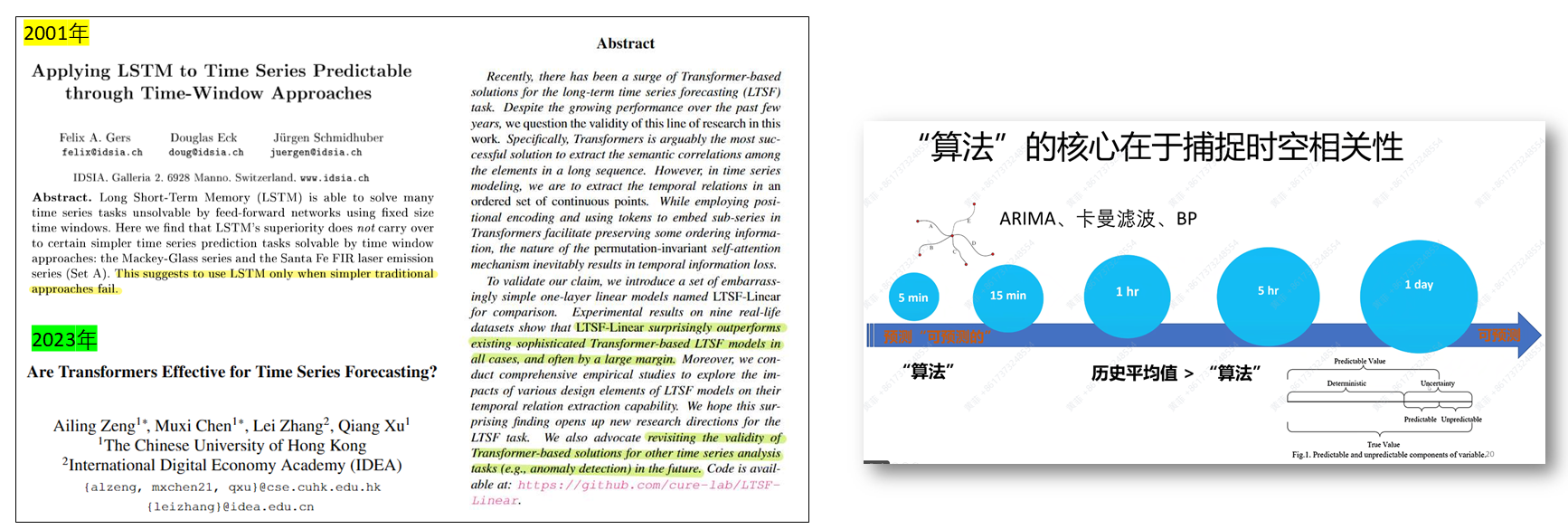
In 2001, an investigation into LSTM research revealed that on certain sequence prediction tasks solvable with temporal sliding-window methods (such as the Mackey-Glass and Santa Fe laser sequence benchmarks), complex modeling did not always yield predictive gains.

Similarly, a 2023 study (Are Transformers Effective for Time Series Forecasting?) discovered that while Transformers excel at long-sequence semantic modeling, the essence of time-series forecasting lies in sequential point-to-point ordering, whereas the permutation invariance of self-attention can cause temporal information loss.

At times, the linear assumptions of LTSF-Linear proved closer to the actual rhythm of the data itself—a phenomenon that echoes the philosophy of GWR in spatial domains, where over-assuming global spatial homogeneity risks masking local heterogeneity.

Returning to trend, seasonality, and dependency decay, these methods originate from economic data induction and exhibit strong transferability.

However, if temporal resolution shifts or sequence modalities change, the manifestations of these patterns shift accordingly: for daily or longer-period sequences, historical averages may suffice; whereas in high-frequency fluctuations sampled at 5 or 15-minute intervals, algorithms truly demonstrate their ability to capture spatiotemporal dependencies.

Much like the Modifiable Areal Unit Problem (MAUP) in geography—where altering map aggregation scales reshapes statistical outcomes—changing temporal resolution determines what we manage to capture and what we miss. Time and space exhibit striking consistency in this regard.

This serves as a reminder that the “capturability” of regularities is not dictated purely by model complexity, but rather depends on the temporal-spatial modality, scale, and internal structure of the data.

The Spatiotemporal (Un)Predictability of Data#

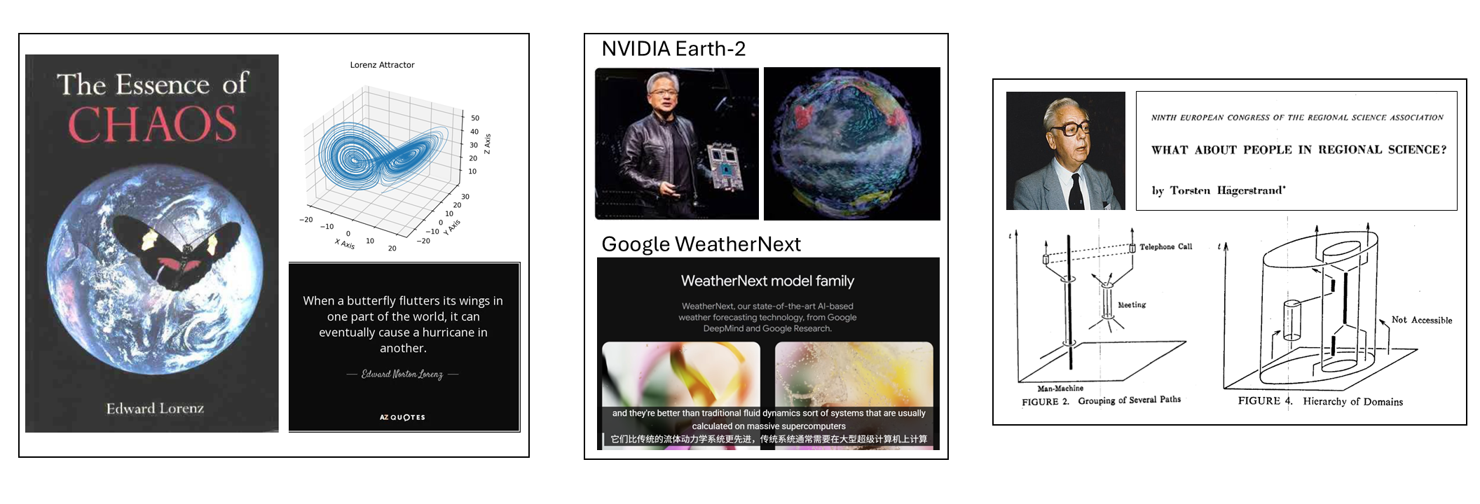
Intuitively, even if we fed every available piece of data into a deep learning model, it could never truly “foresee everything.”

Complex systems are exquisitely sensitive to initial conditions, and the interplay of space and time can generate non-linear amplification effects. Take weather: minuscule perturbations can trigger rainstorms or tempests, with impacts evolving temporally and diffusing spatially with distinct gradients—traits laid bare by chaos theory.

Yet in the context of simulating the Earth, NVIDIA’s Earth-2 and Google’s WeatherNext seem to have captured a “macroscopic order” amidst massive spatiotemporal datasets—not striving to reconstruct the trajectory of every wind gust or the landing spot of every raindrops, but trying to grasp the overall dynamical outline in a statistical sense (note: both frameworks are built upon diffusion models rooted mathematically in Langevin dynamics). While micro-behaviors brim with unpredictability, macroscopic patterns remain learnable and simulable.

This bears a close resemblance to the tenets emphasized by Torsten Hägerstrand’s space-time prism theory: individual movement is constrained not only temporally (daily routines, activity windows) but also spatially (road networks, urban functional zones).

Consequently, even though urban human mobility is a non-linear complex system heavily reliant on spatiotemporal conditions, explicit spatiotemporal constraints imbue predictions with catchable regularities.

In other words, “(un)predictability” is not absolute; it is tied to scale, target, and modeling approach. Even the most complex systems exhibit capturable spatiotemporal dependencies at certain scales and hierarchies.

Thus, the question shifts from whether we can foresee everything to what we actually intend to predict.

From the orbital parameters of Halley’s Comet to the lagged terms of ARIMA models and the hidden states of RNNs, every leap in sequence modeling has been accompanied by an enhancement in our capacity to describe “state.”

Yet within geographic space, the connotation of “state” has grown unprecedentedly rich: it encompasses not only sequential temporal associations but also spatial distance, topology, direction, and semantics.

How to gracefully encode these multidimensional geographic contexts into a language models can understand remains a core hurdle in GeoAI.

Arguably, the boundaries of our exploration into spatiotemporal predictive power depend entirely on the breadth of our imagination regarding spatiotemporal representation.

Author Information & References#

Yuquan Chen
Received his Bachelor's degree from Taiyuan University of Technology and is currently a Master's student in Surveying Engineering (Class of 2024) at the Department of Urban Spatial Information Engineering, Shenzhen University.
Research Interests: GeoAI, POI Deduplication and Configuration.

Guolong Li
Received his Bachelor's degree from Shandong University and is currently a Master's student in Artificial Intelligence (Class of 2023) at the Department of Urban Spatial Information Engineering, Shenzhen University.
Research Interests: GeoAI, Geospatial Data Representation Learning.

Fei Huang
Ph.D. Candidate (Class of 2022), Department of Urban Spatial Information Engineering, Shenzhen University.
Research Interests: GeoAI, Geospatial Tokenization, Human Mobility Generation, Geospatial Data Representation Learning.

This chapter was written by Yuquan Chen, Guolong Li, and Fei Huang with the assistance of AI tools (GPT-5, Gemini 2.5 Pro). Illustrations used in the text are sourced from the Internet.

The cover image was generated by Jimeng AI with the prompt: In the style of Salvador Dalí’s surrealist painting “The Persistence of Memory.” Linear feel, distant landscape, a small robot looking upward, retro, textured, color blocks, gazing at time, blurred outlines. Abstract, fantastical, color blocks, warped time, time lines. Impressionist background, colors, whimsical and dreamy, floating time, clocks drifting in the sky, another clock distorted and fallen to the ground.

References#

1. Temin, P., & Voth, H. J. (2004). Riding the South Sea Bubble. American Economic Review, 94(5), 1654–1668.

2. Wikipedia. (n.d.). Hidden Markov model. Retrieved September 20, 2025.

3. Elman, J. L. (1990). Finding structure in time. Cognitive Science, 14(2), 179–211.

4. StatQuest with Josh Starmer. (2022, July 11). Recurrent neural networks (RNNs), clearly explained!!! YouTube.

5. Dive into Deep Learning. (n.d.). 8. Recurrent Neural Networks. Dive into Deep Learning 2.0.0 Documentation.

6. Ahmed, N. A. (2022, November 10). Vanishing/Exploding Gradients in Deep Neural Networks. Comet.

7. Hochreiter, S., & Schmidhuber, J. (1997). Long short-term memory. Neural Computation, 9(8), 1735–1780.

8. Chung, J., Gulcehre, C., Cho, K., & Bengio, Y. (2014). Empirical evaluation of gated recurrent neural networks on sequence modeling. arXiv:1412.3555.

9. Jonte Dancker. (n.d.). A brief introduction to recurrent neural networks. Towards Data Science.

10. Sutskever, I., Vinyals, O., & Le, Q. V. (2014). Sequence to sequence learning with neural networks. Advances in Neural Information Processing Systems, 27.

11. Minhaz Chowdhury. (2024, September 5). Exploring encoder-decoder architecture with LSTMs. Medium.

12. Nir Arbel. (2019, March 15). Attention in RNNs: Understanding the mechanism with a detailed example. DataDrivenInvestor.

13. Bahdanau, D. (2014). Neural machine translation by jointly learning to align and translate. arXiv:1409.0473.

14. Wikipedia. (n.d.). Attention (machine learning). Retrieved September 20, 2025.

15. Luong, M. T., Pham, H., & Manning, C. D. (2015). Effective approaches to attention-based neural machine translation. arXiv:1508.04025.

16. U-Air: When urban air quality inference meets big data.

17. Are Transformers Effective for Time Series Forecasting?

18. Geographically and Temporally Neural Network Weighted Regression.

19. The geography of parameter space: An investigation of spatial non-stationarity.

20. Autoformer: Decomposition Transformers with Auto-Correlation for Long-Term Series Forecasting.

21. A Time Series is Worth 64 Words: Long-term Forecasting with Transformers.

22. What about people in Regional Science?

Proofread by: Fei Huang