Before diving into the dazzling array of modern artificial intelligence architectures, let us return to the starting point where a pivotal leap first took place. Here, a seemingly humble structure—the Multi-Layer Perceptron (MLP)—took a vital step forward. Like a stroke of genius, it infused algorithms with theoretically boundless expressive power for the very first time, unveiling a vast “promised land” before our eyes. And what guides us across this terrain, drawing wisdom from raw data, is the powerful engine operating behind the scenes: Backpropagation. In this chapter, we will deconstruct these two foundational concepts together. They are the keys that unlock the doors to all subsequent complex models, and the linchpin to understanding how AI evolved from finite, rigid rules to infinite creativity. No matter how magnificent future architectures become, they are all built upon this very same bedrock.

The First Building Block of Intelligence: Multi-Layer Perceptron (MLP)#

One of the fascinating things about history is that the seeds of many great contemporary innovations were often planted in the distant past. This is certainly true of the very first building block of modern deep learning: the Multi-Layer Perceptron (MLP). Today, it serves as the foundation for virtually every complex model, yet its name and original inspiration trace back to a grand—albeit once thwarted—vision from the last century.

The Perceptron: Born from Biological Inspiration and a Grand Vision#

Coined in the 1950s, the term “Perceptron” cleverly blends its biological inspiration with the technological zeitgeist of its era. We can break the word down into two parts to understand its meaning.

1. “Percept”

Rooted in psychology, this forms the core of the name. Its inventor, Frank Rosenblatt, was a psychologist whose grand ambition was not merely to build a calculator, but to use electronic circuits to simulate how biological neurons learn in the brain. In cognitive science, a “percept” refers to the internal mental impression or representation formed after an organism receives sensory information (such as sight or sound) and processes it in the brain. The machine Rosenblatt created was designed to mimic this exact process: taking in raw input data and learning how to classify it. Thus, the root “Percept” directly reflects the machine’s core function—simulating biological perception and recognition.

2. “-tron” (Electronic Device)

This suffix is a hallmark of its time. In the mid-20th century, amidst rapid advances in electronics and atomic energy, “-tron” became a highly fashionable ending used to name cutting-edge, powerful electronic or scientific instruments—think “Electron” or “Cyclotron.” Attaching “-tron” to an invention instantly gave it a high-tech, futuristic aura.

Put the two parts together, and the meaning of Percep-tron becomes crystal clear: an electronic machine built for perception. Not only did the name accurately capture its function, but it also bore the unmistakable imprint of an era brimming with boundless optimism and imagination about “electronic brains.”

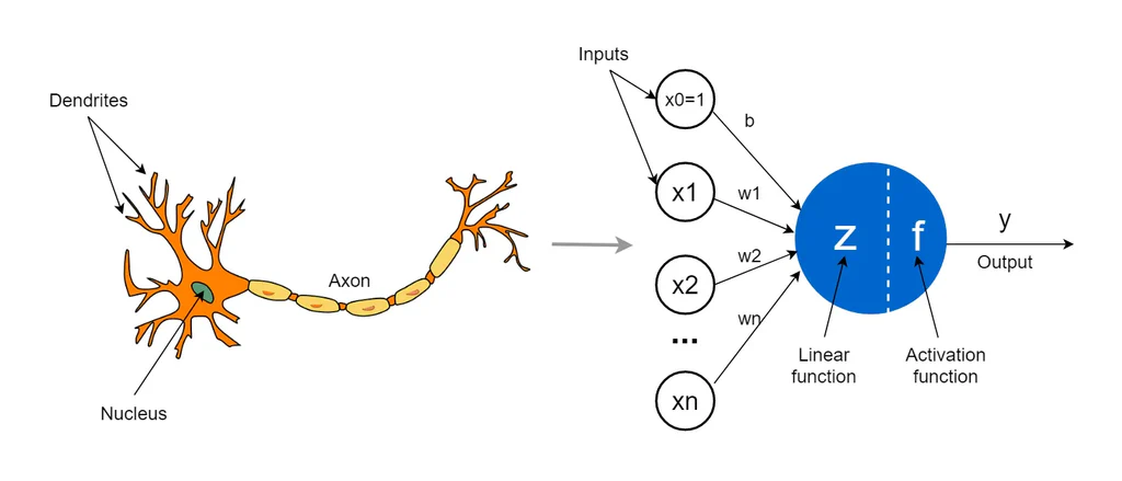
Yet, in stark contrast to this rosy vision was its tragic fate: in 1969, Marvin Minsky and Seymour Papert published Perceptrons: An Introduction to Computational Geometry, proving that such single-layer networks could not even learn the simple XOR (exclusive OR) function. This splash of cold water extinguished enthusiasm for “neural networks” almost overnight. Research funding was virtually frozen, steering the trajectory of AI research toward Symbolicism for well over a decade.

Components and Principles of an MLP#

Structurally, the original Perceptron can be understood as a linear layer immediately followed by a step function. However, researchers soon realized that the step function itself suffered from critical limitations (which we will explore in detail in the upcoming section on backpropagation), preventing the model from scaling into deeper, more complex architectures. Overcoming these limitations led to a series of key improvements that gave birth to the MLP we know today. Its core architecture consists of four main elements: foundational linear layers, activation functions that endow the model with non-linearity, a layer-stacking mechanism that creates network depth, and a final layer that integrates information to produce the output.

A basic MLP takes in input data (a feature vector representing the object of study, typically denoted as x) and processes it. An MLP is generally structured as follows:

1. Linear Layer

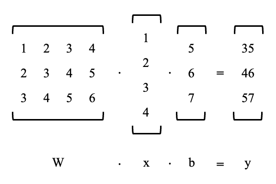
This performs a linear transformation on the data, which can be thought of as a matrix-level upgrade of the simple linear function y=kx+b. Its general formula is:

2. Non-Linear Activation Function

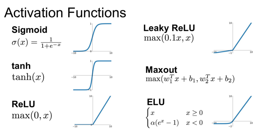
This applies a simple or complex non-linear transformation to the output of the previous step, introducing non-linearity into the model so that it can learn and fit functions far more intricate than mere linear relationships. Common activation functions include:

• The classic Sigmoid
• The simple and widely used ReLU
• Many other specialized variants

3. Stacking

The combination of Linear Layer → Non-Linear Activation from steps 1 and 2 can be viewed as a single fundamental network layer. By stacking and repeating this combination multiple times, we can construct a “deep” neural network capable of modeling hierarchical relationships ranging from simple to highly complex.

4. Final Linear Layer

After passing through a series of hidden layers, the data typically flows into a final linear layer. Its job is to consolidate all the high-level features learned by the preceding layers and map them to the target output dimensions required by the task (for example, outputting the score for each class in a classification task).

The Core of the Magic: What Difference Does Non-Linearity Make?#

If the linear layer handles the primary linear transformation and the non-linear activation function merely clips or bends its output, why can’t we just use linear layers alone? Why is it mandatory to insert a non-linear activation function in between?

The answer hides right in the name—non-linearity. No matter how complex the matrix operations inside a purely linear layer may seem, stacking multiple linear layers on top of one another is mathematically equivalent to using just a single linear layer. Consider the following derivation:

What happens when two linear layers are stacked directly?

This shows that two stacked linear layers have the exact same expressive power as a single, standard linear layer.

However, once we insert a non-linear activation function in between, the picture changes completely:

Because of the intervening non-linear activation function, this expression can no longer be collapsed into a single linear layer.

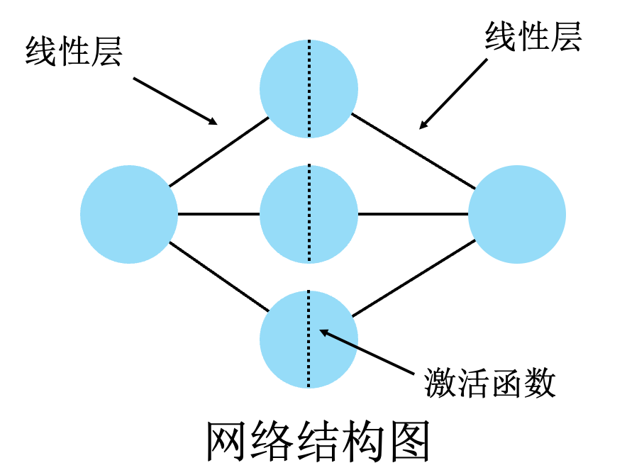
Let’s use a simple linear function example to get an intuitive feel for how introducing a non-linear activation function transforms a model’s representational power:

1. A linear function y=kx+b gives us infinitely extending straight lines.
2. A non-linear activation function, such as the widely used ReLU, truncates these lines—flattening one part to 0 while leaving the other part equivalent to a ray (half-line).
3. Now, we have a rich collection of rays that can be freely combined. By applying another linear transformation to scale, shift, and sum these rays—stitching them together—we obtain a piecewise linear curve (polygonal line).
4. And a piecewise linear line with enough inflection points (bends) can approximate any smooth curve we desire with arbitrary precision.

• Extending the 1D linear function y=kx+b to the high-dimensional y = Wx + b may look more abstract, but geometrically it simply upgrades lines into “hyperplanes.” The network still traces out complex functional relationships in much the same way.
• Note that this specific geometric intuition uses the ReLU activation function as an example. Other non-linear activation functions bend straight lines in different—and sometimes less visually obvious—ways, but the underlying essence remains identical: bending straight lines (linear mappings) into non-linear mappings so we can break free from the trap where “a combination of straight lines is still a straight line,” enabling the network to fit all kinds of curved relationships.

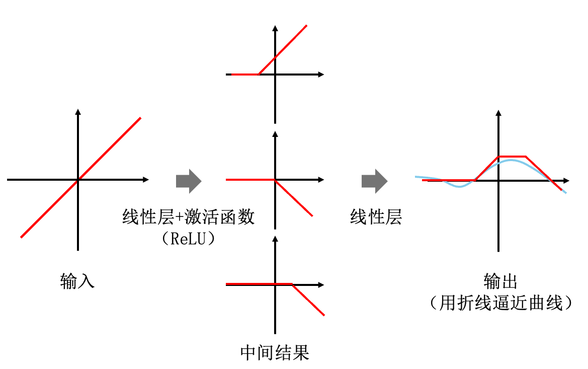
That is the magic of non-linearity. Superimposing straight lines only ever yields another straight line, but combining rays (or the curves produced by other activation functions) allows us to sketch out intricate curves stroke by stroke. After all, most real-world problems involve much more than simple linear relationships; complex challenges almost always exhibit deep non-linearity.

In fact, behind this simple metaphor of “sketching curves with folded lines” lies a remarkably powerful mathematical principle: the Universal Approximation Theorem. This theorem tells us:

In theory, a neural network with just a single hidden layer (i.e., the Linear Layer – Activation Function – Linear Layer architecture we just introduced) possesses the capability to approximate any complex continuous function to any desired degree of accuracy—provided we give it enough neurons (infinite width, rather than the 3 shown in our toy example) and use a non-linear activation function.

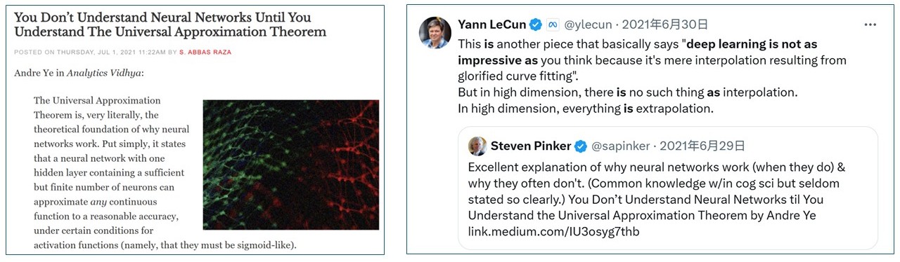
Of course, “infinite width” is strictly a theoretical ideal. In reality, we cannot build a linear layer with infinite parameters because both computing power and memory are finite. Yet this does not stop the MLP from being an extraordinarily useful foundational tool. Returning to our analogy, practical constraints simply mean we have fewer inflection points at our disposal. Our folded line might not hug the true curve as flawlessly as it would in theory, but in most cases, a “good enough” approximation is more than sufficient to get the job done admirably. Accepting a bit of unavoidable error and moving forward—isn’t that true for both life and modeling alike?

The Learning Engine Powered by Backpropagation: How Do Models Get Smart?#

By now, looking at the static skeleton of an MLP, you should have a clear sense of why it holds the potential to fit complex functions. However, an even more crucial piece of the puzzle remains: how do we actually set all those parameters? Starting from random initialization, how does a network adjust itself step by step through exposure to data until it finally learns to solve a problem?

No heavy math is required here. In this section, we will build an intuitive feel for how parameters cooperate to form a powerful learning engine capable of predicting targets.

Loss Function: The Scoreboard Measuring Proximity to the Goal#

First, a model needs to know how well it is doing—and what “doing well” even means. We need a scoreboard to quantify its performance. How should we design this scoreboard? Suppose we are working on a simple prediction task: predicting a target numerical value based on a set of conditions. Our model offers its best guess—the predicted value—and waits eagerly for our feedback: How was my prediction? How should I adjust? Meanwhile, we hold the correct answer in our hands—the true value (ground truth). How do we communicate this gap to the model?

We can frame this as an optimization goal by giving the model an “error score,” where its objective is to make this score as small as possible. The most straightforward idea is to calculate the absolute value of the error: |Predicted Value - True Value|. If the true value is 10 and the model predicts 8, the estimation error (commonly called the “loss”) is 2.

But we can take this a step further: is an egregious error of 4 really only twice as bad as a minor error of 2? Perhaps we want the model to dread making huge blunders. To penalize large errors much more severely, we can amplify extreme mistakes by squaring the difference, defining our “error score” as (Predicted Value - True Value)²:

• For an error of 2, the error score is 2^2 = 4.
• For an error of 4, the error score is 4^2 = 16—making the penalty 4 times as severe!

By squaring the error, our scoreboard becomes hyper-sensitive to major blunders, forcing the model during training to prioritize eliminating its most wildly inaccurate predictions first.

In addition to squaring, we typically evaluate the model across a batch of data points simultaneously and compute their average error. By combining averaging and squaring, we have just co-designed one of the most ubiquitous and powerful loss functions in machine learning. Its formal name is Mean Squared Error (MSE), and its core philosophy is to define a more sensible learning objective by disproportionately penalizing large errors. Beyond MSE, different tasks call for different loss functions. For instance, Cross-Entropy Loss is the standard choice for classification problems, whereas Mean Absolute Error (MAE)—which skips the squaring step—is favored in scenarios where robustness against extreme outliers is desired. Naturally, many more specialized loss functions exist for specific tasks, each brimming with clever design insights waiting for you to explore.

Backpropagation: A Layer-by-Layer Command Relay System#

Alright, we have an overarching goal (minimize the error score), but a neural network contains thousands—or even billions—of parameters. Which ones should we tweak, and in what direction?

This calls for an efficient command relay system. In deep learning, this system is the famous Backpropagation algorithm.

Don’t let the technical name intimidate you; its function is remarkably intuitive: starting from the final error score, it works backward layer by layer in an automated process that tells every single parameter in the network, “On the next step, you should nudge yourself a little higher, or a little lower.”

Imagine a massive team collaborating on a project. After reviewing the final deliverable, the boss (the optimizer) issues a blunt overall verdict: “No good—this final metric is way off target (the loss is too high)!”

Backpropagation acts like a magical internal chain of command that instantly breaks down this vague top-level verdict at each organizational layer, passing actionable feedback down to every individual contributor. When the pressure to improve reaches a team leader at any given layer, an intricate four-step process unfolds:

1. Analyze and Strategize: First, the team leader inspects their own unit’s plan against the directive from above, quickly identifying which specific variables under their control contributed most negatively to the final outcome. They form an initial assessment: “To improve the overall metric, I need to raise Value A and lower Value B—and fixing B is the higher priority.”

2. Self-Adjustment: Next, acting on this assessment, the leader immediately tweaks Values A and B in their plan. In technical terms, this is called updating the parameters.

3. Relay Downward: The team leader knows full well that their unit’s output is built upon proposals submitted by their subordinates (the preceding layer). Therefore, while adjusting their own parameters, they must also pass concrete instructions down the line so the subordinates can help make the new plan succeed: “Hey, for my revised plan to hit its target, the value of XX you’re feeding me needs to be a bit smaller—that will help me the most!”

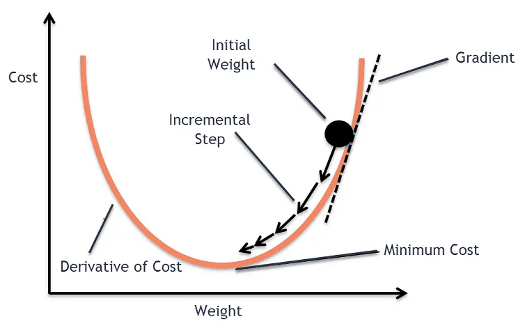
4. Iterate Continuously: A single round of adjustments is never a one-and-done fix; it is merely the beginning of continuous optimization. This is the exact essence of Gradient Descent, illustrated below: the entire organization repeats the cycle of “receive feedback → fine-tune across the board” over and over. Much like a ball rolling down a hill, it doesn’t teleport to the valley floor in a single bound; at every step, it senses which direction slopes downward (computing the gradient) and rolls a small step in that direction (updating the parameters). Through thousands of such iterations, the team’s master plan is gradually polished to near perfection.

The “Backpropagation” Party: Who Didn’t Get an Invite?#

For this magical command relay system to function smoothly, every component must obey one golden rule:

Every mathematical operation in the network must be differentiable.

The “team leaders” from our analogy rely on the mathematical tool of differentiation to calculate precisely how a tiny nudge to their parameters will affect the final outcome. The magnitude and direction of this effect—known as the slope (or derivative/gradient)—form the exact basis for their adjustment strategy.

Now, let’s consider the everyday operation of rounding to the nearest integer. Suppose a “Rounding” team leader tries to use differentiation to figure out how to tweak its internal parameters. Here is what it runs into:

• Almost everywhere, the calculated slope is strictly 0. Mathematically, this tells the unit: “No matter how you tweak your input slightly, it has zero effect on the final output.” The command relay system falls completely silent, leaving the network with no clue which way to move.
• At those exceedingly rare boundary points (such as 3.5), the slope abruptly spikes to infinity. This signal is so violent that it effectively crashes the entire command system.

Thus, the fatal flaw of rounding is that the feedback it provides is either dead silence (zero slope) or a catastrophic explosion (infinite slope), completely severing the chain of command.

Contrast this with our go-to activation function, ReLU. For all positive inputs, ReLU provides a wide-open highway with a constant slope of 1, ensuring that instructions always receive clear, stable, and effective feedback. While signals for negative inputs are truncated to zero, improved variants like Leaky\ ReLU go a step further by preserving a tiny, non-zero slope on the negative side as well, ensuring the communication line never goes completely dead. The key takeaway is that the ReLU family guarantees a viable path for gradient signals to travel, whereas rounding bricks up every doorway.

This is the exact fundamental reason why the original 1950s Perceptron failed to scale. It used the Heaviside step function—a pure, rigid “cliff”—as its activation function. That design made gradient-based learning impossible at the time. Only when the step function was later replaced by smooth or piecewise-linear alternatives like Sigmoid and ReLU was the spark of deep learning reignited.

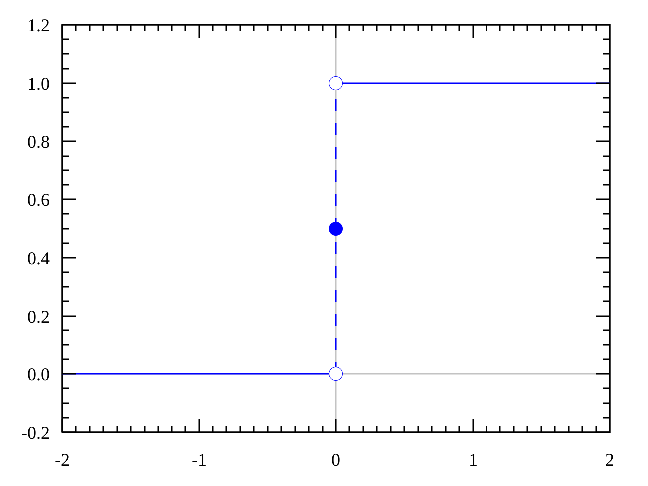
Finally, it is worth emphasizing that this grand party called “Backpropagation” is not hosted exclusively for the MLP. In fact, it is a universal celebration across the entire realm of deep learning. Every sophisticated model we will encounter in later chapters—whether designed for images, audio, or text, and no matter how exotic its architecture—aspires to secure an invitation to this party. And differentiability is the mandatory dress code printed on every single invitation. Once you grasp this, it becomes clear why, despite the dizzying evolution of model architectures, the underlying learning principle remains remarkably unified.

Powerful and Universal, Yet Still Not Enough#

Congratulations! If you have followed along this far, you have successfully navigated the most central—and often most bewildering—conceptual heartland of deep learning. Let’s do a quick recap: we met the foundational building block known as the Multi-Layer Perceptron (MLP), and saw that its true power stems not from any single component, but from the alternating stack of linear layers and non-linear activation functions. This deceptively simple recipe gives the model the ability to approximate any curve using piecewise linear segments, backed by the formidable Universal Approximation Theorem. At the same time, we equipped this static structure with a complete learning engine: designing a loss function to define “good vs. bad,” using backpropagation to efficiently distribute blame for the total error across every parameter, and leveraging gradient descent so the model can iteratively refine itself from data. Differentiability, meanwhile, serves as the foundational rule of the game that keeps this entire intricate machine running.

Yet a few nagging questions remain: if the MLP is already so “universal,” why are there so many other guests at the deep learning party? And why did Steven Pinker point out in his tweet that, despite the guarantees of the Universal Approximation Theorem, neural networks still “so often don’t” work?

Since a sufficiently large MLP (guaranteed by the Universal Approximation Theorem) can fit any complex function, and virtually every problem in the universe can ultimately be formulated as a complex functional mapping, is the MLP the ultimate answer to everything?

—In theory, yes. In practice, however, the story is far less simple. Much like physics at the dawn of the 20th century, dark clouds still hover above this seemingly complete theoretical edifice. In the upcoming Section 2.1, we will lift the curtain on why: using images as an example, we will examine the practical bottlenecks that MLPs run into despite their ironclad theoretical guarantees. This will lead us directly to the classic architecture born to overcome those very limitations—the Convolutional Neural Network (CNN)—and we will witness how it ignited the golden age of deep learning sparked by the ImageNet competition. In the chapters that follow, we will venture even further to see how deep learning has evolved specialized architectures tailored to the unique structures of different real-world problems.

Author Information & References#

Guolong Li
Received his Bachelor's degree from Shandong University and is currently a Master's student in Artificial Intelligence (Class of 2023) at the Department of Urban Spatial Information Engineering, Shenzhen University.
Research Interests: GeoAI, Geospatial Data Representation Learning.

This chapter was written by Guolong Li with the assistance of AI tools (Google Gemini 2.5 Pro). Some illustrations used in the text are sourced from the Internet.

References#

1. Lefkowitz, M. (2019). Professor’s perceptron paved the way for AI – 60 years too soon. Cornell Chronicle.

2. Pramoditha, R. (2021). The Concept of Artificial Neurons (Perceptrons) in Neural Networks. Towards Data Science.

3. Jadon, S. (2018). Introduction to Different Activation Functions for Deep Learning. Medium.

4. Ye, A. (2020). You Don’t Understand Neural Networks Until You Understand The Universal Approximation Theorem. Medium.

5. Crypto1. (2025). Gradient Descent Algorithm: How Does it Work in Machine Learning?. Analytics Vidhya.

6. Wikipedia. (n.d.). Step Function. Retrieved September 7, 2025.

7. Header Image Reference

Proofread by: Fei Huang