The history of evolution has a curious habit of repeating itself. Over 500 million years ago, one of the key catalysts behind the Cambrian explosion was the birth of vision. When living organisms opened their eyes for the very first time, an evolutionary “arms race” in cognitive capability began, ultimately shaping complex brains. Hundreds of millions of years later, in 2012, AlexNet achieved a watershed victory in the ImageNet visual recognition challenge. From that moment on, deep learning—spearheaded at the time by computer vision—stepped into the spotlight and embarked on its own “Cambrian moment.” Across a gulf of half a billion years, it seems an astonishing coincidence: vision once again served as the spark that ignited a “singularity.”

Plunging from the structured data that MLPs were long accustomed to—where features are distinct and largely self-contained—straight into a vibrant world composed of high-dimensional pixels feels much like Alice tumbling down the rabbit hole into a Wonderland where familiar rules and order instantly dissolve. Here, every individual pixel is like a silent playing-card soldier: meaningless in isolation, yet holding the secrets of the entire kingdom within its collective arrangements and combinations. The finely crafted tools we built for the old world suddenly appear clumsy and powerless, because they no longer face a handful of clear-cut “features,” but rather a chaotic yet deeply interconnected ocean of pixels. In this chapter, let us step down this wondrous rabbit hole together and explore how the Convolutional Neural Network (CNN) became the “eyes” that enabled early artificial intelligence to truly “see” the world.

Convolutional Neural Networks: From Visual Neurons to the Dawn of Deep Learning#

At the end of the previous chapter, we left behind a pivotal question: since the Universal Approximation Theorem theoretically guarantees the formidable expressive power of the MLP, why does an MLP struggle so mightily when confronted with image data, necessitating a brand-new architecture? Ian Goodfellow and his co-authors answered this question directly in their classic textbook Deep Learning:

The universal approximation theorem means that regardless of what function we are trying to learn, we know that a large MLP will be able to represent this function. We are not guaranteed, however, that the training algorithm will be able to learn that function.

How should we make sense of this? Imagine that our MLP model now has to answer a seemingly simple question: is the main subject of a given 128 \times 128 image a flower, or something else entirely?

An MLP must first flatten the image into a 128 \times 128 = 16384-dimensional vector, and then recognize and assemble its contents from the ground up—a cluster of pixels forms an edge, a set of edges forms a petal, petals arrange themselves into a blossom, and together with the stem and stamen, the model can finally conclude with confidence that the picture shows a flower rather than a blade of grass or a cat.

That hierarchical assembly is complex enough on its own, yet an MLP must also overcome two additional hurdles:

• Adjacent pixels arranged in a certain pattern might signify a corner or an edge, whereas pixels scattered randomly across the image with the exact same values probably mean nothing at all. An MLP is forced to sift through a astronomical number of futile combinations just to learn which dimensions are spatially adjacent and closely related, and which combinations are meaningless.
• What makes a petal a petal depends primarily on the relative pattern of its pixels, not on whether it appears in the top-left or bottom-right corner of the image. Because an MLP has no mechanism to share parameters across different input dimensions, it must independently build recognition capabilities for virtually every single position in the image—even when those capabilities are similar or downright identical.

These two hurdles do not invalidate the Universal Approximation Theorem; rather, they pose a formidable challenge to the learning process itself. Ideally, we should bake two fundamental truths directly into the model—that neighboring dimensions are strongly correlated, and that the same recognition capability can be reused across different locations—rather than forcing the network to rediscover these facts from scratch. Formally, we can express these two properties of images as:

• Spatial Locality: Relationships between pixels are not created equal; the meaning of a pixel is primarily tied to its immediate neighbors.
• Translational Symmetry (or Translation Invariance/Equivariance): Regardless of where a local pattern appears in an image, its core underlying meaning remains unchanged.

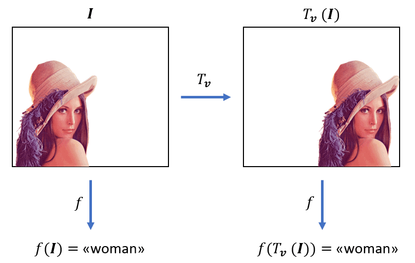
Any neural network designed to process images ought to reflect these requirements directly in its architecture, instilling the natural laws of image data into the model as an innate prior. How can we achieve this? Fortunately, neurobiological discoveries made decades earlier had already pointed the way.

Convolution Operations Inspired by Neurobiology#

In their pioneering research during the 1960s, neurobiologists David Hubel and Torsten Wiesel discovered that when a cat views different objects, neurons in its primary visual cortex fire in response to specific patterns within specific regions of the visual field (Hubel & Wiesel, 1962). For instance, certain neurons respond strongly to vertical lines, while others are tuned to horizontal lines. Even more intriguingly, each of these neurons monitors only a small localized patch of the visual field rather than the entire scene—a property known as a “Receptive Field.” This groundbreaking discovery later earned them the 1981 Nobel Prize in Physiology or Medicine.

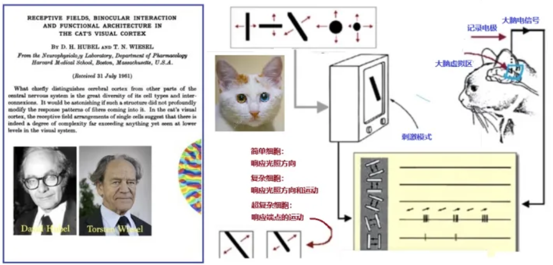
Inspired by this biological insight, Yann LeCun and his colleagues proposed the Convolutional Neural Network (CNN) for handwritten character recognition in 1989. By 1998, they had developed the more mature LeNet-5 architecture, widely regarded as the foundational cornerstone of modern CNNs.

The design of a CNN ingeniously emulates three key characteristics of the biological visual system:

• Local Receptive Fields: To match the spatial locality of images, each neuron only needs to attend to a small local patch of the image—much like how we examine a picture piece by piece rather than taking in every minute detail all at once. When a CNN recognizes a cat, for example, it might first detect a furry ear, then spot the whiskers, and only later assemble them into a complete cat face.
• Weight Sharing: To match the translational symmetry of images, the exact same feature detector (called a convolutional kernel or filter) can be reused across all locations in an image—just as our ability to recognize a cat’s ear doesn’t change whether the ear appears in the upper-left or lower-right corner. This drastically reduces the number of parameters in the network: instead of training a separate detector for every single position, sharing a single set of weights across the board does the trick.
• Pooling Operations: A CNN periodically compresses its feature maps, retaining the most salient information while reducing data dimensionality. This is akin to how human vision grasps key features without memorizing every pixel-level detail: whether a cat’s ear is tilted slightly to the left or right, we still effortlessly recognize it as a cat’s ear.

Together, these three innovations form the core strengths of CNNs, directly addressing the structural laws of images discussed earlier. Specifically, local receptive fields allow the network to process local spatial structures efficiently; weight sharing slashes model parameters by orders of magnitude by reusing convolutional kernels across the image; and pooling operations bolster the network’s robustness against minor shifts and distortions by preserving only the most essential features.

It is precisely this design that makes CNNs exceptionally adept at handling data with spatial structure. Not only can they “read” images, but they also learn features hierarchically from simple to complex, mirroring the biological visual system. Built upon this inspiration and exploration, CNNs vastly expanded the horizons of neural networks and ushered in the magical moment that came to symbolize the birth of modern deep learning.

1. LeNet-5#

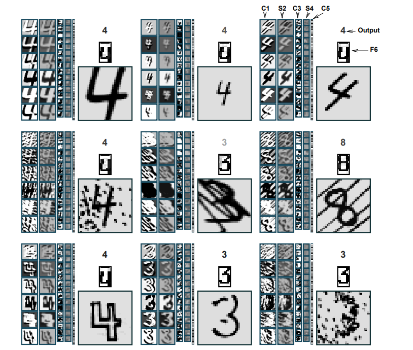
Proposed by Yann LeCun’s team in 1998, LeNet-5 was designed primarily for handwritten digit recognition. Compared to the pure MLP architecture covered in the previous chapter, LeNet-5 can be thought of as a “Convolutional Feature Extractor + MLP Decision-Maker.” By combining local receptive fields, weight sharing, and pooling operations, the convolutional feature extractor effectively distills the raw spatial information of an image into a compact vector representation. Freed from confronting complex pixel grids head-on, the MLP at the end can focus entirely on making the final classification decision.

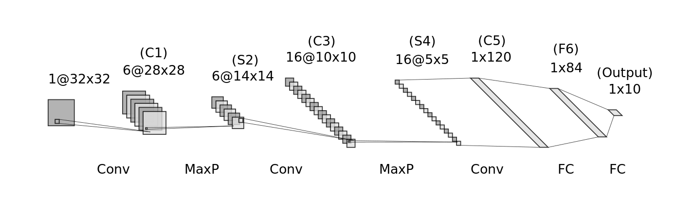
It is worth noting that LeNet-5 was far from a purely academic exercise. As the first CNN deployed in large-scale commercial applications, it helped banks automatically process millions of handwritten checks throughout the 1990s, marking a major early triumph in the commercialization of neural networks. However, in an era that strongly favored traditional statistical machine learning methods, the success of LeNet-5 did not immediately spark widespread adoption across the research community. Even after proving the potential of CNNs, this technical trajectory remained largely sidelined for over a decade—until 2012, when the field reached a decisive turning point…

2. AlexNet: The Crossroads of an Era#

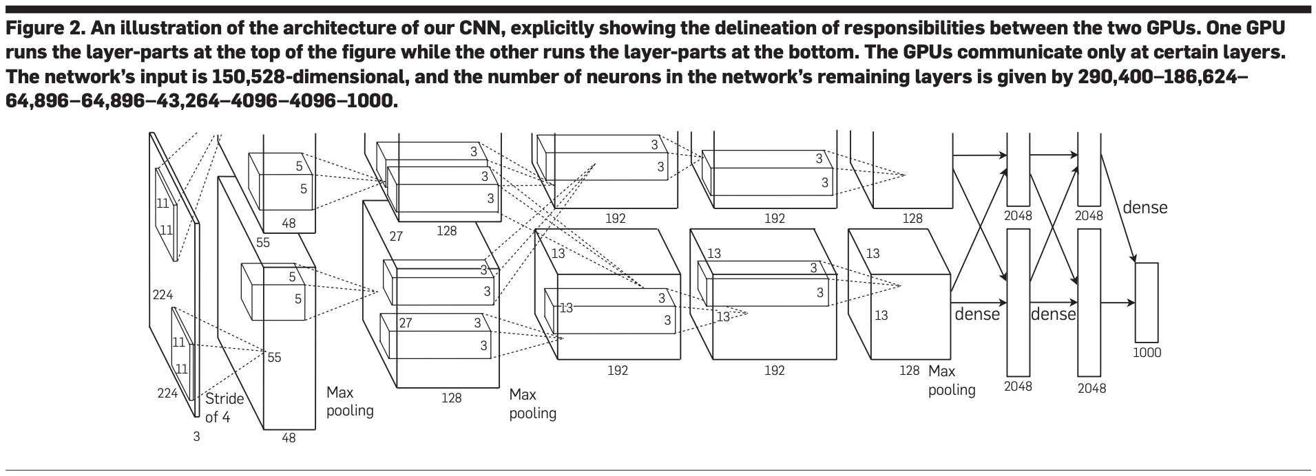
Launched in 2009 by Fei-Fei Li and her team, the ImageNet Large Scale Visual Recognition Challenge (ILSVRC) quickly became the gold-standard benchmark for evaluating computer vision algorithms due to its massive scale and formidable difficulty. The competition required algorithms to accurately classify millions of real-world photographs into 1,000 distinct categories—an exponential leap in complexity compared to the 10 handwritten digits tackled by LeNet-5.

In the 2012 competition, AlexNet entered the arena! Following the CNN paradigm pioneered by LeNet-5, it scaled up to a significantly deeper architecture (5 convolutional layers and 3 fully connected layers) to meet the demands of ImageNet. The results were nothing short of seismic: AlexNet achieved a Top-5 error rate of just 15.3%, whereas the runner-up—relying on traditional computer vision methods—lagged behind at 26.2%. Such a commanding lead proved beyond a shadow of a doubt the transformative potential of deep learning for complex visual recognition tasks.

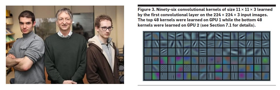
First and foremost, AlexNet’s victory was a triumph for the CNN architecture itself. Its performance demonstrated that the “Convolutional Feature Extractor + MLP Decision-Maker” paradigm established by LeNet remained the right answer for complex visual problems once scaled up in size and depth.

Yet the historical significance of AlexNet extends far beyond architecture alone. Its triumph was the culmination of several converging factors, formally establishing the modern paradigm of deep learning research. Alongside a deeper CNN structure, AlexNet creatively repurposed GPUs—originally built for 3D graphics rendering—to accelerate neural network computation, unlocking unprecedented computing power for training larger and deeper models.

At the same time, its success relied on the maturation and deployment of several pivotal training techniques: adopting the ReLU activation function to dramatically speed up training, and introducing Dropout regularization to combat overfitting. Equally indispensable was the massive open-source ImageNet dataset, which acted as the decisive catalyst. Not only did it supply vast amounts of “fuel” for model training, but more importantly, it validated and cemented the “data-driven” methodology at the heart of modern deep learning.

Now, let us bring our focus back to the CNN itself and examine the specific components it uses to meet the demands of image data.

Dissecting the CNN Architecture: Synergy Between Two Core Modules#

Starting from biological first principles, we have seen why CNNs are designed the way they are. Now let us switch to an engineer’s perspective and dissect this precision machine to see how these concepts translate into concrete components working together along an efficient pipeline—from raw pixels to high-level insights.

In many classic textbooks and tutorials, a CNN is described as a sequential chain of layers: “Input Layer,” “Convolutional Layer,” “Pooling Layer,” “Fully Connected Layer,” and “Output Layer.” This nomenclature originated in the early days of CNN research, when pioneers coined distinct terms for these newly introduced image-processing components to highlight how sharply they differed from traditional MLPs.

Today, however, as modular thinking has become standard across deep learning, this historical terminology often creates unnecessary confusion. Calling the endpoints the “Input Layer” and “Output Layer,” for example, merely describes their position in the pipeline without conveying their computational nature—the former is simply raw, unprocessed data, while the latter is typically just the final linear projection and probability normalization step of the classifier.

Similarly, the term “Fully Connected Layer” overemphasizes its contrast with “locally connected” convolutional layers, obscuring its true identity: our familiar friend the MLP module, which is responsible for final decision-making. Clinging to these historical labels fragments the functional logic of a CNN as an integrated system and no longer serves modern intuition well.

Let us therefore set aside those rigid labels for a moment and deconstruct the CNN from a higher-level, functionally grounded perspective—namely, the “Convolutional Feature Extractor + MLP Decision-Maker” framework we introduced earlier.

Input Data#

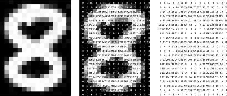
The starting point of our pipeline is a digitized raw image. Whether it is a handwritten digit or a street-view photograph, to a computer it is nothing more than a numerical grid (or “tensor”) of pixel intensities—such as a 28 × 28 × 1 matrix for a grayscale image. This is the raw material we are about to refine.

Convolutional Feature Extractor#

This is the very soul of a CNN. Its sole mission is to refine the raw pixel matrix into a Feature Vector rich in high-level semantic information. This module is built primarily from two repeatable, stackable components:

1. Convolutional Component

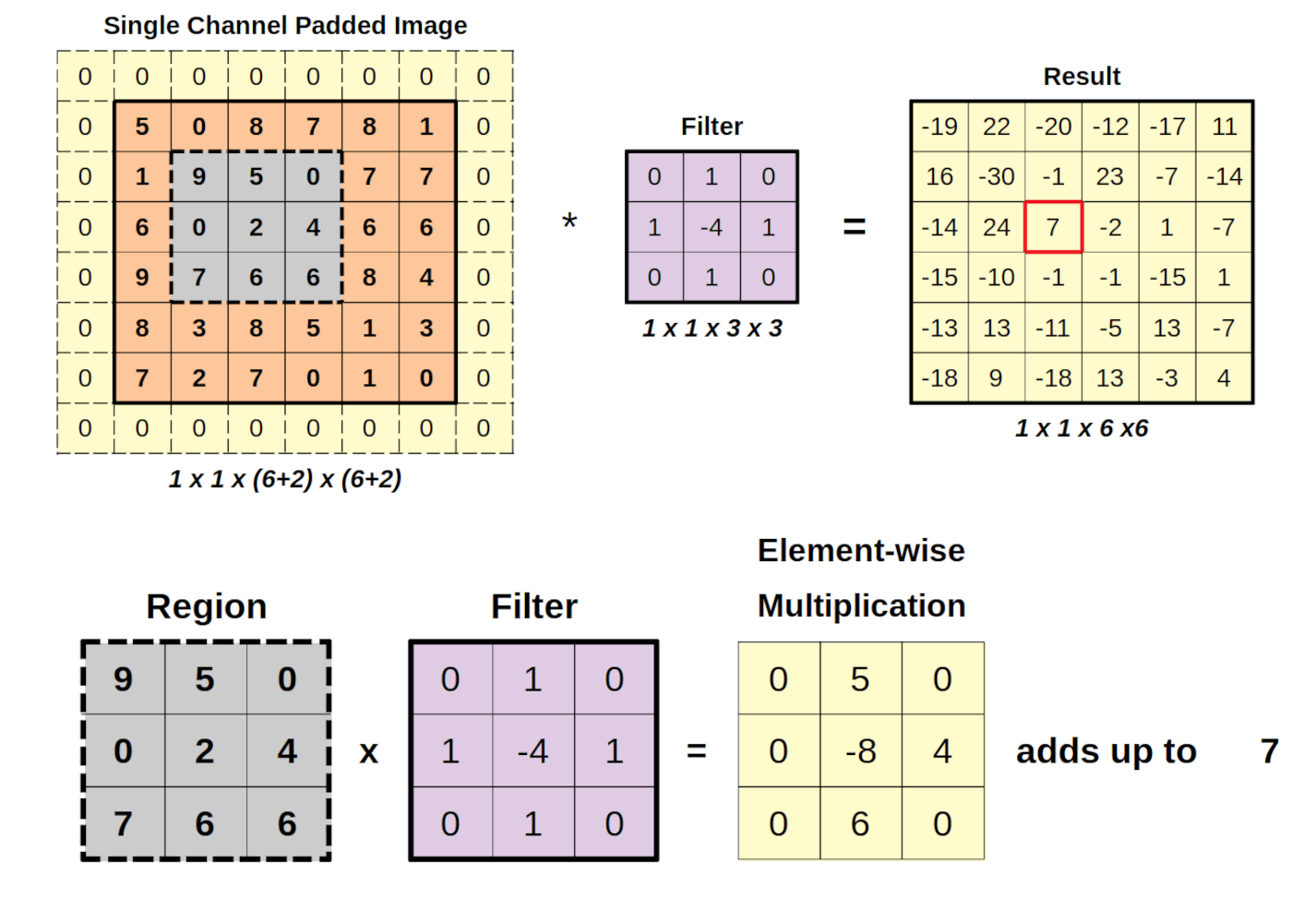
This is the primary workhorse of feature extraction. Using multiple small, shared local pattern detectors (convolutional kernels or filters) that slide across the image, it scans for foundational patterns such as edges, corners, and textures, producing a set of Feature Maps.

2. Pooling Component

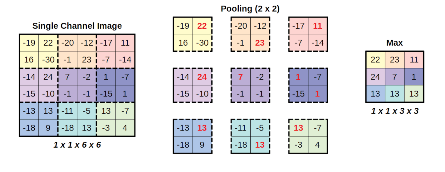
This acts as the able assistant in feature extraction. By performing “intelligent compression” (such as Max Pooling) on the feature maps, it retains the most prominent feature signals while reducing spatial dimensions, endowing the model with tolerance (robustness) to minor shifts and deformations of objects.

The real magic lies in the emergent power of stacking itself. When we stack these relatively simple “Convolution–Pooling” blocks on top of one another repeatedly, a remarkable hierarchical dependency emerges:

• Shallow convolutional components may only detect primitive “edges” and “short strokes.”
• Middle convolutional components assemble those strokes into “arcs” or “corners.”
• Deep convolutional components combine those “arcs” and “corners” further into recognizable object parts, such as a “closed loop.”

The number of these stacked core blocks is referred to as the Depth of the network. Through layer upon layer of progressive refinement, the feature extractor ultimately outputs a highly abstract, information-dense vector representation that serves as the basis for downstream decision-making.

MLP Decision-Maker#

Once the feature extractor completes its analysis, this highly abstract feature vector is handed over to our old friend—the MLP Decision-Maker. Its job is straightforward: take the “analytical report” delivered by the feature extractor and, based on those high-level features, learn how to render a final verdict.

Take digit classification as an example. The report submitted by the feature extractor effectively reads: “In the upper half of this image, I detected a ‘closed loop’ feature; in the lower half, I also detected a ‘closed loop’ feature…” Upon reading this report, the MLP classifier brings its strength in feature integration into play, synthesizes the evidence, and outputs a vector of raw “likelihood scores” (Logits) for each candidate category.

For instance, it might assign a very high score to the output neuron corresponding to the digit 8.

Probabilistic Output#

While the raw scores (logits) produced by the MLP reflect the relative likelihood of each class, they are not immediately intuitive. If the digit “6” gets a score of 46 and “8” gets a score of 58, what does that actually mean in terms of confidence? To answer this, we typically apply a standalone Softmax function at the very end. Its role is to convert arbitrary raw scores into a clean, interpretable probability distribution that sums to 1 (100%).

Ultimately, the model can report back clearly: “I estimate there is a 98% probability that this digit is an ‘8’, a 1% probability that it is a ‘6’… Therefore, my final prediction is 8.”

By now, you have a solid grasp of the foundational structure and inner workings of CNN models. Yet as mentioned earlier, a major reason AlexNet excelled on a massive thousand-class benchmark like ImageNet was the simultaneous leap in dataset scale, network capacity (width and depth), and GPU computing power.

Interestingly, looking back from today’s era of Large Language Models, it is that exact same recipe—internet-scale text corpora paired with hundreds of billions of model parameters—that gave rise to ChatGPT and the “intelligence” emerging under Scaling Laws.

Back when AlexNet first burst onto the scene, however, the infrastructure for deep learning was still in its infancy, and the theory and methodology for effectively training “deeper, larger” networks were far from settled. Researchers at the time naturally began to ask: Can we push even further than AlexNet? By making networks deeper and deeper, can we ultimately unlock the deepest truths hidden within visual data?

VGG and ResNet: An Odyssey into “Depth”#

Following AlexNet, researchers established “increasing network depth” as a primary avenue for boosting model performance, launching an intensive wave of exploration into deep network architectures. Along the way, the emergence of VGG and ResNet provided crucial methodological breakthroughs for how to build and train deep CNNs.

1. VGG: A Systematic Exploration of Modular Depth#

In the wake of AlexNet, the Visual Geometry Group (VGG) at the University of Oxford chose a direct, disciplined path to explore network depth. Guided by a philosophy of simplicity and uniformity, VGG demonstrated that simply stacking standardized “building blocks”—specifically, small 3 \times 3 convolutional kernels—to greater depths was enough to construct extraordinarily powerful networks. This elegant modular design philosophy remains a cornerstone of neural network engineering to this day.

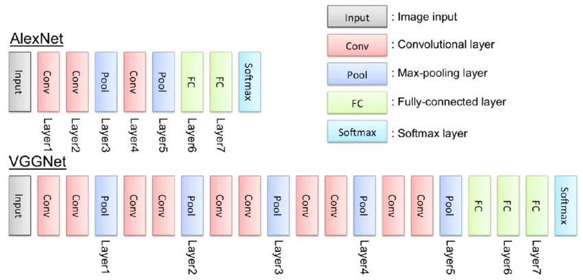
While the VGG architecture achieved tremendous success in the 2014 ImageNet challenge, perhaps its greatest historical contribution was exposing the bottleneck of brute-force depth. When researchers attempted to stack VGG-style layers even deeper (e.g., beyond 20 layers), a perplexing phenomenon known as network degradation set in: deeper networks actually performed worse—even on the training set—than their shallower counterparts.

This was not caused by overfitting; rather, extreme depth itself introduced fundamental optimization difficulties during training. VGG’s experiments laid this paradox squarely before the entire research community.

2. ResNet: A Structural Innovation for Training Deep Networks#

One of the primary culprits behind the network degradation encountered by VGG is the vanishing gradient problem. In the command relay system (backpropagation) we discussed in the previous chapter, when a network has too many layers, the feedback signal traveling backward from the final output gradually attenuates layer by layer, leaving the earliest layers near the input virtually unable to update effectively.

Confronted with this roadblock, Kaiming He and his colleagues—then at Microsoft Research Asia—proposed a brilliant architectural solution: ResNet (Residual Neural Network).

Their core insight was simple yet profound: forcing a stack of layers to learn a brand-new, complex mapping directly from input A to output B is hard; however, asking it to learn only the small incremental adjustment—the “residual” (or difference) between A and B—is vastly easier.

To realize this idea of learning residuals, ResNet introduced the Skip Connection (or Shortcut Connection). It creates a direct bypass pathway that carries the input of a block untouched around the intermediate convolutional layers and adds it directly to the block’s output. This express highway ensures that both forward information and backward gradient signals can flow unimpeded across layers, effectively alleviating vanishing gradients and network degradation in deep architectures.

Here, it is worth clarifying an important distinction: ResNet is not a brand-new breed of convolution, nor is its signature innovation—the Skip Connection—exclusive to CNNs. Rather, it is a universal architectural design principle applicable across virtually all families of deep neural networks (including modern Transformers). Yet it was the ingenious application of this universal idea to deep convolutional networks at the time that broke the “curse of depth” plaguing the entire field in one fell swoop.

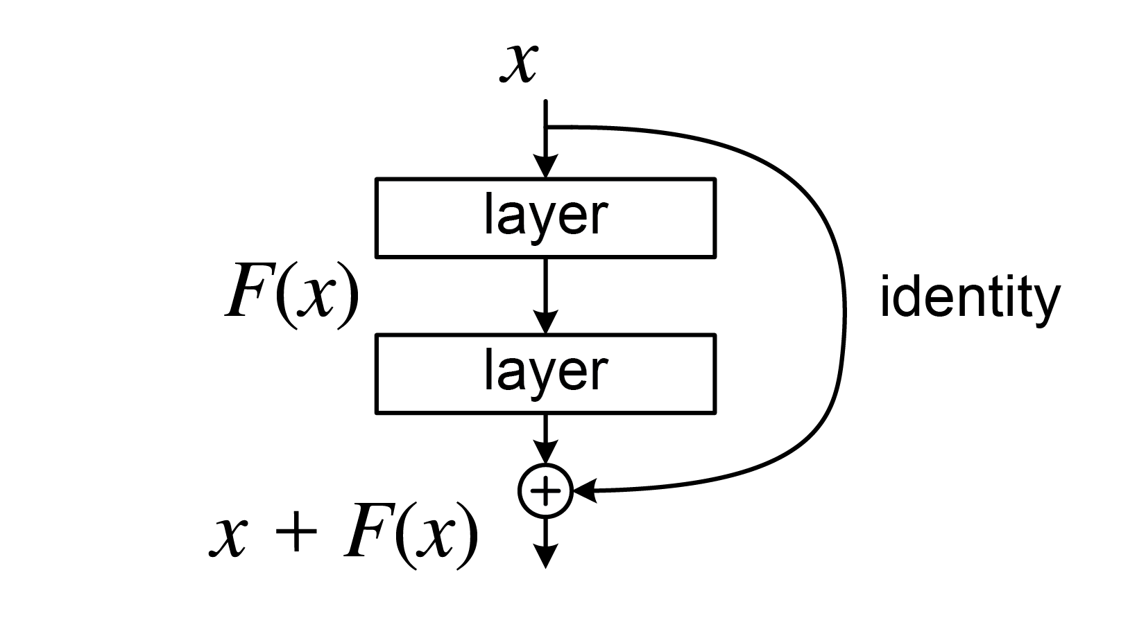
The birth of ResNet shattered the ceiling on network depth, making it possible to train ultra-deep networks spanning hundreds or even thousands of layers. Rather than merely piling on more layers, ResNet answered the fundamental question of how to construct depth effectively.

VGG’s exploration defined the problem, and ResNet’s ingenuity supplied the answer. Together, their dialogue forms one of the most defining chapters in the evolution of deep learning architectures.

The Boundaries of CNNs and New Horizons#

Up to this point, we have traced the pivotal opening journey of deep learning: from the “universal approximation” theory of MLPs, to the elegant adaptation of CNNs for visual data, and finally to pushing the limits of performance through network depth. Compared to everyday computational methods, this toolkit is already remarkably powerful—perhaps even overwhelmingly intricate.

Yet is our journey over? Even if we restrict our scope strictly to visual problems, is our prized weapon—the deep Convolutional Neural Network—truly invincible? For better or worse, the answer is no. Standing atop this peak and looking ahead, new challenges emerge on the horizon, prompting us to ask three fundamental questions:

1. The Limitation of “Field of View”

The bedrock of a CNN is spatial locality—it assumes that relationships between immediately adjacent pixels matter most. A convolutional kernel acts like a narrow searchlight whose size dictates its field of view, relying on network depth to stack these local glimpses layer by layer until the model eventually “sees” the whole picture.

But this raises a natural question: where does “local” end? In a photograph of a cat, the head and the tip of the tail may lie far apart in pixel space, yet conceptually they belong to the exact same creature. Does a CNN’s rigid adherence to local neighborhoods become an innate shackle when trying to grasp such long-range dependencies? If we could design a mechanism that lets a model dynamically learn where to focus on local details and where to forge global connections across the entire image, could it achieve visual understanding that surpasses fixed convolutional filters?

2. The Absence of “Time”

The native battlefield of a CNN is 2D space; it excels at parsing how pixels are laid out across a flat plane. Yet the real world is not frozen in a static frame. When our data is inherently sequential—such as a video clip, an audio recording, or a passage of text—the dimension of time takes center stage.

Just as the spatial arrangement of pixels defines an image, the sequential order of words defines the meaning of a sentence. When confronted with sequential data, doesn’t relying on an MLP for isolated judgments, or using a CNN over a fixed “time window,” risk losing the vital context of flowing information? Do we need a fundamentally new architecture—a network capable of remembering the past and anticipating the future—specifically built to meet the challenge of time?

3. The Diversity of “Domains”

Even within the realm of images, intrinsic data characteristics vary wildly across domains. LeNet-5 dealt with structurally simple handwritten digits, and ImageNet comprises millions of everyday natural photographs—whereas geospatial analysis confronts urban streetscapes and satellite remote sensing imagery with entirely distinct scales, projections, and spectral textures.

Can we rely on a single, one-size-fits-all CNN architecture to conquer every domain? Or do specialized visual domains call for more tailored, domain-aware model designs?

We will dive into the third question in detail in the very next section. As for the first two cliffhangers—achieving a global field of view across space, and endowing models with memory and predictive power across time—we will uncover those answers in the exciting chapters to come.

Applications of CNNs in Spatial Data Processing#

Amid the rapid rise of deep learning, CNNs served as the true starting point for bringing geospatial data analysis into the deep learning era. They were the first to demonstrate transformative potential on classic image-based spatial datasets—most notably remote sensing imagery and street-view imagery. Not only did CNNs dramatically boost accuracy across these tasks, but they also prompted the geospatial community to ponder a deeper question: Should geospatial data be treated differently from everyday natural images in computer vision, inspiring image-processing paradigms specifically tailored to the unique properties of geographic space?

Below, we examine two major categories of image-based spatial data to illustrate how CNNs are applied in geospatial data processing.

Applications of CNNs in Street-View Imagery Processing#

In everyday computer vision, most standard benchmark images center on a single primary subject—a cat, a flower, or a car—where the primary goal is simply to identify “what it is” based on the object’s appearance.

Street-view imagery is likewise captured from a ground-level, “human-eye perspective,” yet its content is never confined to a single isolated object. Instead, it encompasses an entire complex urban scene: roads, buildings, trees, vehicles, and pedestrians all appear simultaneously, captured by cameras mounted on moving vehicles or carried by pedestrians to document the real-world environment along city streets.

When processing street-view imagery, it is not enough to merely recognize individual elements; we must also understand the spatial relationships between them.

For instance, the exact same car carries very different semantic meanings depending on whether it is parked legally by the curb or driving down an active lane; likewise, whether a building faces a main thoroughfare or a quiet back alley has a vastly different impact on the character and vitality of the streetscape.

When a street-view photo shows pedestrians strolling along a sidewalk, bicycles neatly parked at the curb, and storefronts lining both sides of the street, the spatial combination of these elements immediately conveys the impression of a vibrant, bustling neighborhood.

CNNs excel at “deconstructing scenes” from the complex pixel grids of street-view imagery, turning visually cluttered photographs into computable urban elements and quantitative indicators that support research and practice in public space planning and urban governance.

Seeing “What Is There” — Object Detection#

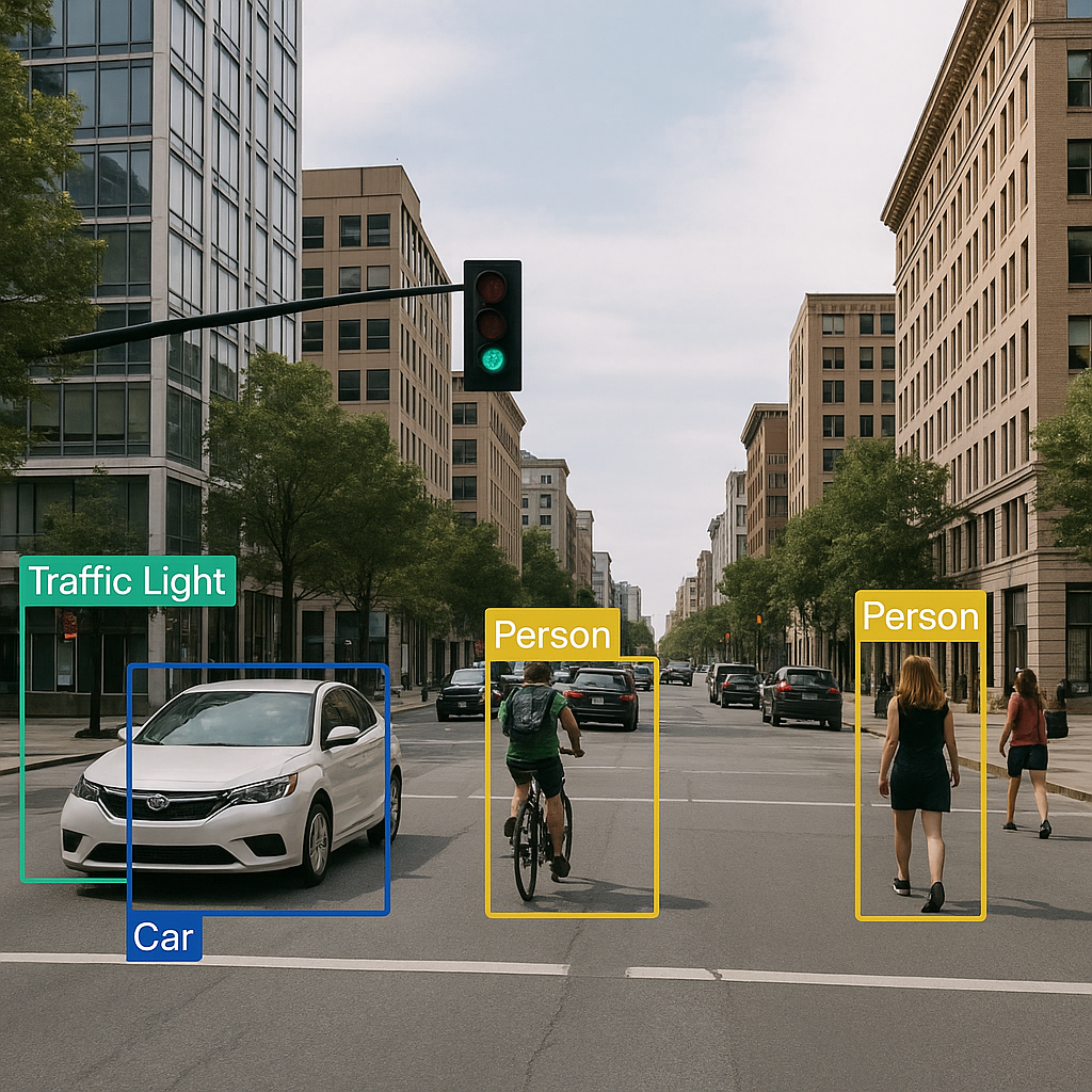
The most foundational task in street-view analysis is identifying “what objects are present” in the scene—a task known as Object Detection. It mirrors how we naturally scan our surroundings while walking down a street: “There’s a car, a pedestrian, and a streetlight over there.”

Powered by CNN-based architectures (such as the classic YOLO family of models), a computer can automatically detect diverse urban elements in street-view imagery—vehicles, pedestrians, traffic lights, street signs—and draw bounding boxes around each one (see left figure below). In doing so, an otherwise cluttered street photograph is transformed into a structured, itemized “inventory of street elements.”

These detections not only help planners tally traffic volumes, but can also be used to monitor sidewalk obstructions, evaluate street-level safety, and even provide real-time environmental perception for autonomous driving systems.

Left: Object Detection (Generated by GPT-5)

Right: Semantic Segmentation (Generated by GPT-5)

Seeing “Where Everything Is” — Semantic Segmentation#

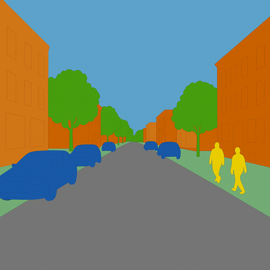
If object detection is about “counting what objects are on the street,” then Semantic Segmentation is like “coloring in the streetscape”—delineating the exact pixel-by-pixel boundaries of every surface and structure.

Using CNN architectures designed for dense prediction (such as the classic U-Net), every single pixel in a street-view image is classified into a semantic category such as road, sidewalk, building, sky, or vegetation (see right figure above), yielding a high-precision “urban semantic map.” From this pixel-level map, researchers can directly compute metrics such as road network connectivity, barrier-free sidewalk continuity, and street-level greenness (Green View Index).

However, standard semantic segmentation only distinguishes between categories, not between individual instances within the same category. Two cars parked next to each other will both be labeled as “vehicle” pixels, without telling us where Car A ends and Car B begins.

Overcoming this requires Instance Segmentation, which not only classifies every pixel but also separates distinct individual objects within the same class. You can think of instance segmentation as marrying the “individual-distinguishing” power of object detection with the “pixel-precise boundary” power of semantic segmentation—enabling finer-grained streetscape analysis for applications like traffic monitoring and autonomous driving.

Notably, in 2023 Meta AI open-sourced the universal foundation model for image segmentation: the Segment Anything Model (SAM). SAM demonstrated an astonishing “segment anything” capability: in principle, it can isolate and segment virtually any object or region in an image—whether common vehicles and pedestrians, irregular tree canopies, patches of sky, or even the narrow gaps between paving stones.

Furthermore, SAM has shown impressive versatility as a foundation for spatial depth and distance estimation. You can try out the interactive online Demo on the official SAM website by uploading your own photos to experience “segmenting anything” firsthand.

Of course, while marveling at breakthroughs like SAM, it also prompts us as geospatial researchers to reflect: now that the computer vision community has built general-purpose models capable of accurately detecting and segmenting objects across street-view and even remote sensing imagery, what should our next scientific frontier be?

Understanding Geometry and Spatial Relationships#

Object detection tells us “what is on the street,” and semantic segmentation maps out “where each category is located.” Yet merely knowing that “there are cars and a road” is not enough; we also need to understand “what the spatial relationship between the car and the road is.”

The key to grasping spatial relationships lies in treating a streetscape as a three-dimensional physical environment rather than a flat 2D photograph. For example, a car positioned on a motor vehicle lane indicates normal traffic flow, whereas the exact same car parked atop a pedestrian sidewalk represents an obstruction and a safety hazard.

Similarly, the geometric interplay between buildings and roadways directly shapes the human experience of a street: when tall buildings tightly flank a narrow street, the space feels canyon-like and oppressive; conversely, lower building heights or wider setbacks create a sense of openness and comfort.

The spatial distribution of greenery matters just as much: a dense overhead tree canopy paired with continuous roadside planting strips significantly enhances pedestrian thermal and visual comfort, whereas scattered, fragmented shrubs rarely achieve the same effect.

Technically, analyzing such 3D relationships typically relies on monocular depth estimation (inferring near-to-far distance relationships from 2D images) and 3D reconstruction (recovering the three-dimensional geometric structure of the street canyon). Armed with these techniques, researchers can quantify urban design metrics such as sky openness, street enclosure, and three-dimensional green volume.

Because these spatial relationships directly shape everyday human experience as well as traffic safety, environmental livability, and public space governance, understanding spatial relationships represents the true core of street-view analysis—taking us from merely cataloging “what elements exist on a street” to comprehending “how those elements come together to form a living urban space.”

Applications of CNNs in Remote Sensing Imagery Processing#

Whereas natural photographs and street-view images are mostly captured from a close-range “human-eye perspective,” remote sensing imagery views the Earth from a top-down “bird’s-eye (or god’s-eye) perspective.” A single satellite scene can span everything from a neighborhood to an entire metropolis, or even数百 (hundreds of) square kilometers of terrain.

When confronting imagery collected from satellites, manned aircraft, and drones—characterized by vast spatial coverage and dramatic variations in scale—the problems a model must solve differ fundamentally from recognizing a cat or a car.

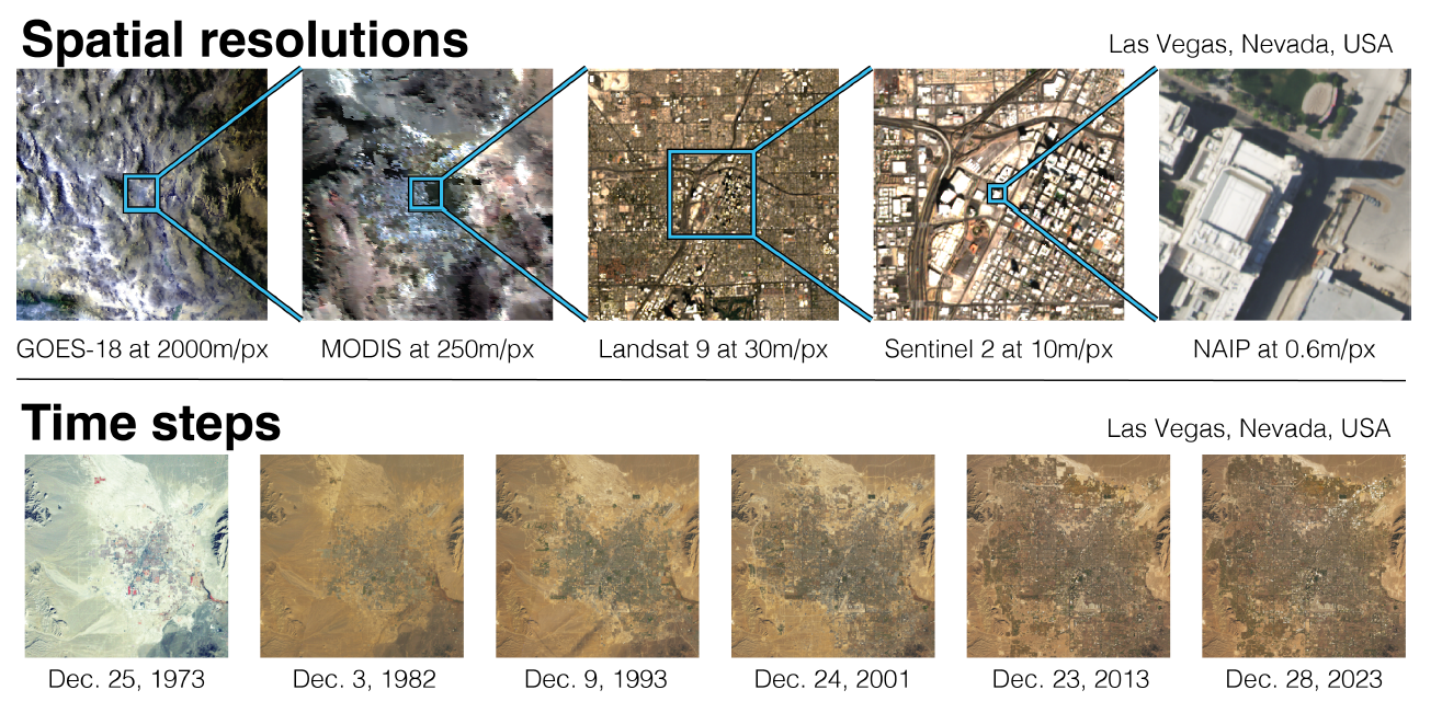
In remote sensing imagery, semantic meaning is governed not only by visual texture, but also by spectral signatures, temporal dynamics, and broader geographic context. Mangrove forests, for instance, grow almost exclusively along tropical intertidal coastlines, whereas permanent snow and ice cover will never appear in low-latitude lowlands.

Consequently, the application of deep learning models to remote sensing imagery has undergone a progressive “spatialization” over time. Broadly speaking, this evolution has moved from initially learning purely from local image textures, to implicitly capturing spatial relationships via multi-scale spatial context, and finally toward spatially explicit models that directly incorporate geographic coordinates and spatial inductive biases.

From Local Feature Learning to Spatially Explicit Modeling#

1. Early CNNs: Learning from Local Features

When deep learning was first introduced to remote sensing image analysis, models relied primarily on small local convolutional kernels to extract patch-level features. Although the effective receptive field grows as more layers are stacked, the information captured by the model remains confined to a limited spatial neighborhood.

While stacking local filters works well for classifying everyday natural images by capturing local textures and object shapes, remote sensing scenes cover expansive areas with complex spatial structures where semantic meaning depends heavily on large-scale spatial context rather than local texture alone.

Constrained by their limited receptive fields, early CNNs struggled to capture long-range cross-regional dependencies, often resulting in fragmented or spatially inconsistent representations of geographic structures.

2. Leveraging Richer Spatial Context: Pixel-Level Semantic Segmentation and Multi-Scale Modeling

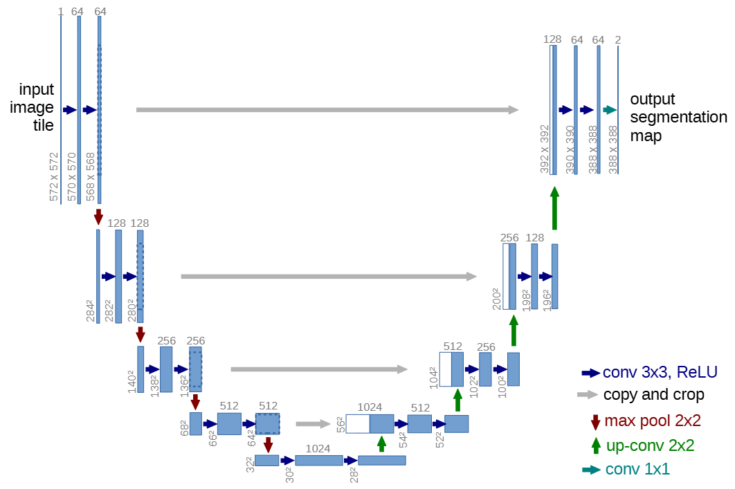
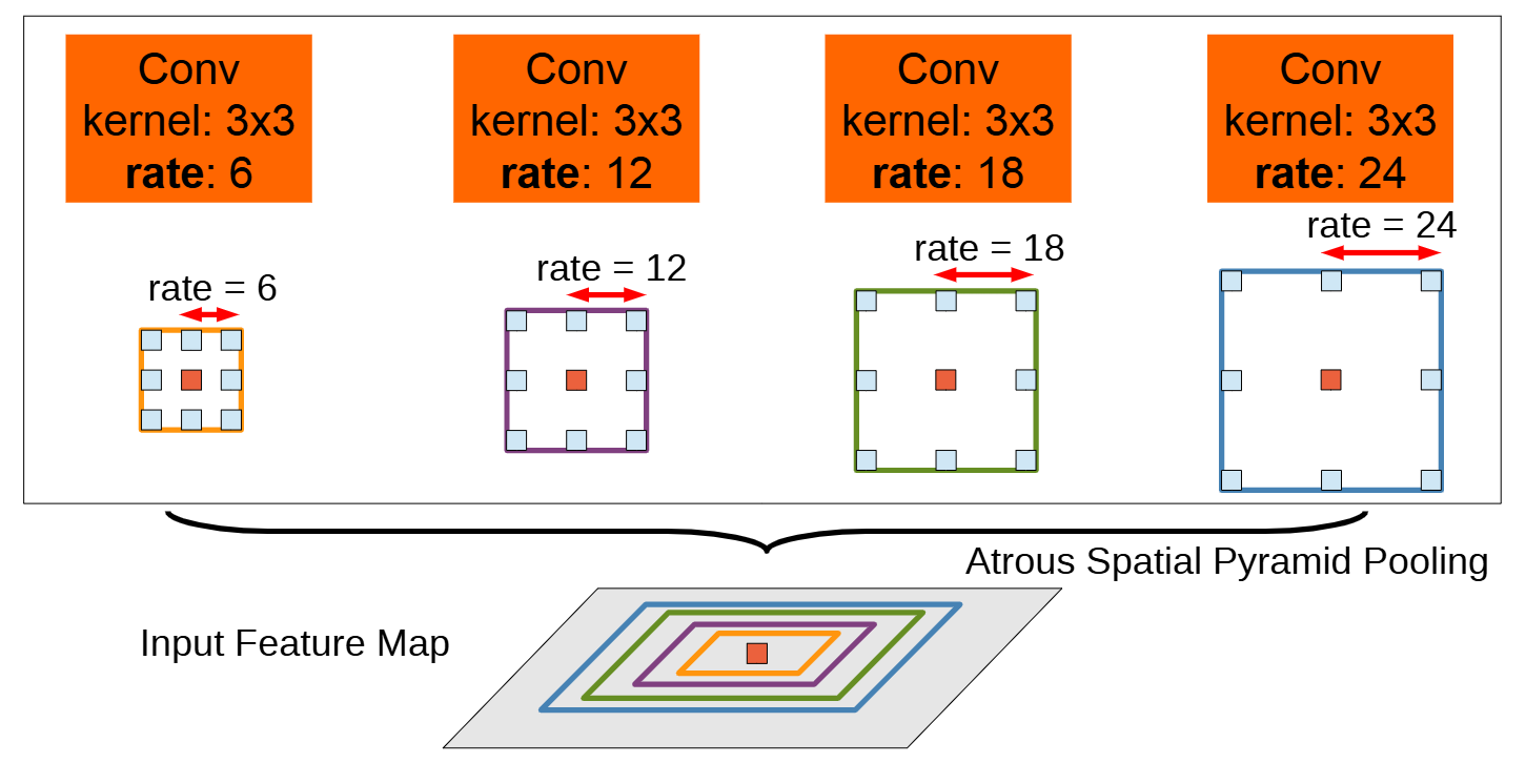
To capture broader spatial context, researchers turned to multi-scale feature fusion and receptive-field expansion techniques. Two classic representatives are U-Net, whose encoder–decoder architecture and skip connections fuse fine local details with high-level global semantics (left figure below), and DeepLab, which employs atrous (dilated) convolutions and Atrous Spatial Pyramid Pooling (ASPP) to observe a scene across multiple spatial scales simultaneously (right figure below).

These designs freed models from viewing imagery solely through a narrow “magnifying glass,” equipping them instead with both a “macro lens” and a “wide-angle lens” at once to capture multi-scale spatial semantics more holistically.

Even at this stage, however, spatial relationships were still learned implicitly: while a model could distinguish buildings from roads, it could not yet explicitly reason about underlying geographic constraints such as network connectivity or topographic rules.

Left: U-Net model architecture (Source: Ronneberger, O. et al.)

Right: Atrous Spatial Pyramid Pooling (Source: Chen, L.-C. et al.)

3. Explicitly Integrating Geographic Knowledge into Models

As remote sensing tasks grew more sophisticated, researchers increasingly recognized that for deep learning models to truly excel in geospatial applications, they needed to “understand space.” In other words, predictions shouldn’t just “look accurate” at the pixel level—they must also be spatially plausible (for example, rivers should not abruptly break into disconnected segments, and road networks should maintain topological continuity).

An early and effective way to inject geographic knowledge into CNNs was concatenating geographic prior channels directly alongside the input imagery. For instance, appending latitude and longitude coordinate grids to the RGB or multispectral channels allows the network to leverage absolute geographic location when learning land-cover distribution patterns.

Beyond absolute coordinates, researchers also incorporate topographic variables (Digital Elevation Models, slope, aspect) as well as precomputed spatial proximity rasters (such as Euclidean distance to the nearest road, river, coastline, or human settlement).

Equipped with these auxiliary inputs, the model no longer relies solely on spectral signatures and visual textures, but can actively exploit geospatial constraints to refine its predictions.

Nevertheless, because standard convolution is fundamentally bound to local grid neighborhoods, it retains inherent limitations when modeling long-range spatial dependencies and non-Euclidean topological relationships. It is precisely these limitations that have driven researchers to explore new architectural paradigms—from Graph Convolutional Networks (GCNs) to Attention Mechanisms—gradually building a much richer modeling ecosystem. (For Graph Neural Networks and Attention Mechanisms, please see the upcoming chapters…)

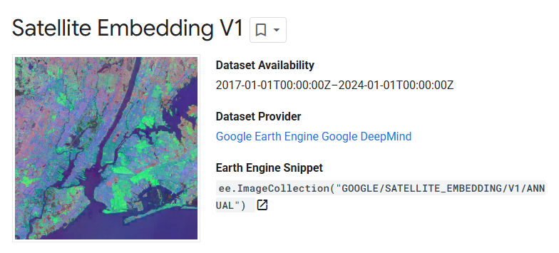
More recently, AlphaEarth Foundations, released by Google DeepMind, has pushed remote sensing image analysis to a new frontier. Rather than training a task-specific model from scratch for a single narrow objective (such as building footprint extraction or land-cover classification), it pre-trains on massive multi-source Earth observation archives—spanning optical imagery, synthetic aperture radar (SAR), climate variables, and terrain data—to learn a universal “Earth representation” (embedding field).

As a geospatial foundation model, AlphaEarth Foundations demonstrates remarkable generalization even in label-scarce regimes, heralding a new era of general-purpose, multimodal Earth intelligence.

Here we use AlphaEarth Foundations merely as a teaser; further advances in geospatial foundation models will be unpacked in detail in later chapters.

Beyond modeling spatial structures, temporal dynamics across time series represent another vital dimension of remote sensing data.

As noted earlier, if a model stops at analyzing static “spatial snapshots,” it risks missing the underlying trajectory of how geographic phenomena evolve over time. Many mission-critical applications—such as crop growth monitoring, dynamic land-cover change detection, and disaster progression modeling—depend fundamentally on time-series modeling.

Capable of retaining memory of the past to forecast the future, the Recurrent Neural Network (RNN) is a cornerstone tool for sequential data processing. In the next chapter, we will first introduce the core principles of RNNs and their key variants, and then explore their applications in multi-temporal remote sensing analysis as well as broader spatiotemporal datasets such as human mobility trajectories.

Author Information & References#

Guolong Li
Received his Bachelor's degree from Shandong University and is currently a Master's student in Artificial Intelligence (Class of 2023) at the Department of Urban Spatial Information Engineering, Shenzhen University.
Research Interests: GeoAI, Geospatial Data Representation Learning.

Qianting Chen
Master's graduate (Class of 2022) in Geographic Information and Smart City, Department of Urban Spatial Information Engineering, Shenzhen University.
Research Interests: Spatialization of Population Attributes.

Shan Hu
Received her Ph.D. from the Institute of Geographic Sciences and Natural Resources Research (IGSNRR), Chinese Academy of Sciences, and is currently a Postdoctoral Fellow at the School of Architecture and Urban Planning, Shenzhen University.
Research Interests: Poverty and Social Inequality Based on Spatiotemporal Big Data.

This chapter was written by Guolong Li, Qianting Chen, and Shan Hu with the assistance of AI tools. Some illustrations used in the text are sourced from the Internet.

The cover image was generated by Jimeng AI with the prompt: Mosaic painting, image divided by dense colorful mosaic tiles, vintage, abstract, oil painting impression, bold color contrast, retro, blurred details. Low-angle view looking up from the mouth of a cave, cave walls covered in blooming flowers. A medieval robot at the cave entrance leaning forward, front view, low-angle close-up of its face.

References#

1. Goodfellow, I., Bengio, Y., Courville, A., & Bengio, Y. (2016). Deep learning (Vol. 1, No. 2). Cambridge: MIT press.

2. Baeldung. (2024). Translation Invariance and Equivariance in Computer Vision. Baeldung.

3. Institute of Physics, CAS. (2024). How Did Cats Inspire the Birth of Artificial Neural Networks? (猫咪怎样启发了人工神经网络的诞生？). Zhihu.

4. Wikipedia. (n.d.). LeNet. Retrieved September 14, 2025

5. Krizhevsky, A., Sutskever, I., & Hinton, G. E. (2012). Imagenet classification with deep convolutional neural networks. Advances in neural information processing systems, 25.

6. Ray, T. (2025). AlexNet, the AI model that started it all, released in source code form - for all to download. ZDNet.

7. Wikipedia. (n.d.). Convolutional neural network. Retrieved September 14, 2025

8. LeCun, Y., Bottou, L., Bengio, Y., & Haffner, P. (2002). Gradient-based learning applied to document recognition. Proceedings of the IEEE, 86(11), 2278-2324.

9. NehaCkumari. (n.d.). MNIST-Handwritten-Digit-Recognition-using-CNN. GitHub.

10. Bangar, S. (2022). VGG-Net Architecture Explained. Medium.

11. Wikipedia. (n.d.). Residual neural network. Retrieved September 14, 2025

12. Segment Anything Research by Meta AI

13. Rolf, E., Klemmer, K., Robinson, C., & Kerner, H. (2024). Mission Critical–Satellite Data is a Distinct Modality in Machine Learning. arXiv preprint arXiv:2402.01444.

14. Ronneberger, O., Fischer, P., & Brox, T. (2015, October). U-net: Convolutional networks for biomedical image segmentation. In International Conference on Medical image computing and computer-assisted intervention (pp. 234-241). Cham: Springer international publishing.

15. Chen, L. C., Papandreou, G., Kokkinos, I., Murphy, K., & Yuille, A. L. (2017). Deeplab: Semantic image segmentation with deep convolutional nets, atrous convolution, and fully connected crfs. IEEE transactions on pattern analysis and machine intelligence, 40(4), 834-848.

16. Brown, C. F., Kazmierski, M. R., Pasquarella, V. J., Rucklidge, W. J., Samsikova, M., Zhang, C., Shelhamer, E., Lahera, E., Wiles, O., Ilyushchenko, S., Gorelick, N., Zhang, L. L., Alj, S., Schechter, E., Askay, S., Guinan, O., Moore, R., Boukouvalas, A., & Kohli, P. (2025). AlphaEarth Foundations: An embedding field model for accurate and efficient global mapping from sparse label data. arXiv preprint arXiv:2507.22291.

Proofread by: Fei Huang