The subject of this chapter is Reinforcement Learning (RL), which may hold the answer. We will trace its origins from classic animal experiments to rigorous mathematical theory—two streams of thought whose convergence gave birth to reinforcement learning—before exploring how deep learning later became its powerful engine. Building on this foundation, how will we achieve Artificial General Intelligence (AGI)? Will Large Language Models (LLMs) alone get us there? By the end of this chapter, a Turing Award laureate’s perspective may offer you a completely different inspiration.

Trial-and-Error and Optimal Control: The Two Intellectual Roots of RL#

To understand how AlphaGo used reinforcement learning to compute an “intuition” that surpassed human grandmasters, we must trace two distinct intellectual lineages. The first is rooted in the observation of biological instinct and seeks to answer: “What is learning?” The second was born of rigorous mathematical deduction and asks: “What is an (optimal) solution?”

These two paths—one centered on trial and error, the other on solving for optimality—appeared to pursue different goals in different domains, yet were ultimately unified within the framework of reinforcement learning.

Learning Through Trial and Error#

The first intellectual thread—trial and error—is ancient and intuitive. It stems from a fundamental observation: how do we, along with the animals around us, learn to navigate and survive in a complex world without an instruction manual? We are not talking about memorizing declarative facts, but rather acquiring actionable wisdom—how to make the right moves in an environment to seek rewards, avoid harm, and achieve goals.

The behaviorist psychologist Edward Thorndike was the first to systematically study this active, goal-directed form of learning. He designed the famous “puzzle box” experiment: a cat trapped inside a box had to perform a specific, non-instinctive action (such as pressing a lever) to open the door and reach food outside. After stumbling upon success by chance, the cat gradually eliminated ineffective movements in subsequent trials, escaping faster and faster.

Thorndike summarized this process as the Law of Effect: responses that are closely followed by a “satisfying state of affairs” become more firmly connected with the situation, so that when it recurs, they are more likely to be repeated; responses accompanied by discomfort have their connections weakened.

This is the fundamental mechanism of trial-and-error learning: an organism actively explores its possibilities, and its behaviors are selected by the consequences they produce in the environment.

B. F. Skinner inherited and substantially expanded upon the Law of Effect. One of his key contributions was replacing the subjective term “satisfaction” with the objective concept of reinforcement.

Reinforcement is precisely defined as any consequence that increases the likelihood of a behavior occurring again in the future. Skinner distilled this basic unit of learning into the “three-term contingency”—a loop consisting of context (discriminative stimulus S^D) — action (response R) — reward (reinforcing stimulus S^R).

From Thorndike’s active trial and error to Skinner’s systematic reinforcement, this intellectual lineage came into sharp focus. Together, they outlined a learning paradigm that neither requires perfect prior knowledge nor presupposes an optimal path. Instead, learning is grounded in direct interaction with the environment—guided by experience and judged by outcomes.

Yet, while this lineage profoundly revealed the nature of learning, it remained a set of elegant qualitative principles rather than a rigorous engineering methodology. Thorndike’s Law of Effect and Skinner’s reinforcement lacked quantitative formulations and concrete computational mechanisms (for example, how to mathematically quantify “satisfaction” or “value”).

This lineage was waiting for a more precise mathematical language to forge these biological observations into computable reality.

Planning and Solving Under Exact Models#

Running parallel to the biological path of groping forward through trial and error was a starkly different intellectual tradition.

Originating in mathematics and engineering in the 1950s and pioneered by figures like Richard Bellman, this second path was not concerned with the biological process of “learning,” but rather with a pure mathematical question:

If a sequential decision-making problem can be completely specified, how do we compute its optimal solution?

The foundational worldview—and formal language—of this lineage is the Markov Decision Process (MDP).

The tractability of an MDP rests on the Markov Property: the future depends only on the present state, and is independent of the past history.

The simplifying power of this assumption is immense. Without it, we would have to condition decisions on the entire history of interactions, causing the state space to grow exponentially over time and rendering the problem computationally intractable. The Markov property compresses an infinitely complex history into a finite, solvable space.

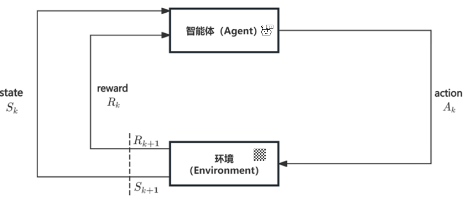
Once an MDP is defined, Dynamic Programming (DP) serves as the core methodology for solving it (assuming both P and R are fully known). The theoretical cornerstone of DP is Bellman’s Principle of Optimality.

The Principle of Optimality states: An optimal policy has the property that whatever the initial state and initial decision are, the remaining decisions must constitute an optimal policy with regard to the state resulting from the first decision.

This can be understood through a simple proof by contradiction: Suppose the optimal route from A to D passes through B. If the “B-to-D” segment were not the optimal path from B to D, we could simply replace it with a better B-to-D route, yielding an overall A-to-D route superior to our assumed “optimal” one—a clear contradiction.

The Bellman Equation is the mathematical embodiment of the Principle of Optimality within the MDP framework.

It establishes a recursive relationship for the ultimate objective—the optimal value function V_*(s) (the maximum expected future return achievable starting from state s).

The Bellman Optimality Equation specifies the condition it must satisfy:

Because of the \max operator, this equation is nonlinear and cannot be solved in closed form all at once. However, it can be solved iteratively using an algorithm called Value Iteration.

Starting from an arbitrary initial guess V_0, the algorithm repeatedly substitutes the current estimate V_k into the right-hand side of the Bellman equation to compute a new, more accurate estimate V_{k+1}:

This iterative process is mathematically guaranteed to converge to the unique optimal value function V_*.

The mathematical route is remarkably powerful and elegant, providing a complete theoretical framework and computational procedure to find a provably optimal solution.

However, the entire edifice of Dynamic Programming rests on one major premise: we must possess a perfect model of the environment.

To run Value Iteration, we must know all the rules of the world in advance—namely, the exact transition probabilities P and reward function R. In the real world, this condition is rarely met.

Herein lies the ultimate dilemma of this tradition: mathematics defines the exact destination we seek, yet demands that we hold a complete map of the world that almost never exists in reality.

The Convergence of Ideas: Barto and Sutton’s Path to the Turing Award#

For decades, these two paths toward understanding intelligence ran in parallel: one rooted in biological instinct (trial and error), rich with insight into experiential learning yet lacking a precise computational language; the other born in the halls of mathematics (optimal control), equipped with a powerful theory of optimality yet hobbled by its requirement for a perfect world model.

The former knew how to learn, but could not compute; the latter knew how to compute, but could not learn in the unknown.

The historic synthesis of these two streams was achieved by Andrew G. Barto and Richard S. Sutton, earning them the 2024 ACM A. M. Turing Award.

Their collaboration personified the marriage of the two intellectual traditions. Barto’s academic background spanned psychology and neuroscience, deeply inspired by biological trial-and-error learning mechanisms. Sutton, Barto’s doctoral student, brought formidable mathematical and algorithmic rigor, carrying forward the optimal control tradition.

Together, they resolved the central impasse: Dynamic Programming (the “solving” route) was bottlenecked because computing the expectation in the Bellman equation required a complete, perfect model of P and R.

Their breakthrough was to replace this uncomputable “expected target” with the very soul of the trial-and-error tradition: real samples obtained through direct interaction with the environment.

Mathematically, this fusion unfolds as follows.

In Dynamic Programming, an update relies on an expectation that cannot be computed without knowing the model:

In Reinforcement Learning, by contrast, the agent interacts with the environment through trial and error to collect a real experience sample (s,a,r,s').

Barto and Sutton’s key insight was to use a sample-based estimated target (such as r + \gamma V(s')) in place of the unknown expected target.

This sample-driven learning adopts an incremental update rule:

Here, \text{Target} is the estimated target derived from actual experience, and \alpha (the learning rate) is the mathematical embodiment of trial and error: we use new experience to correct our current estimate, taking a small step toward the new target.

This powerful idea—solving the Bellman equation via sample estimates—led to one of their most foundational contributions: Temporal Difference (TD) Learning, which elegantly resolves the problem of delayed rewards.

Building on this, they also developed Actor-Critic Architectures, introducing a division of labor between action selection and value evaluation that makes learning substantially more stable and efficient.

These two pivotal concepts, which we will unpack in detail below, form the algorithmic bedrock of modern reinforcement learning.

Beyond these algorithmic breakthroughs, Barto and Sutton made another monumental contribution: codifying and unifying the entire field.

In 1998, they published their seminal textbook, Reinforcement Learning: An Introduction.

Widely regarded as the “bible” of the field, the book unified disparate threads—Dynamic Programming, Monte Carlo methods, and their own Temporal Difference learning—under a single, coherent theoretical framework for the first time.

It established the standard terminology, notation, and core problem formulations that have trained virtually every generation of RL researchers since. (This chapter also draws heavily on their book, particularly its 2018 second edition.)

With their work, the strengths of both intellectual traditions were seamlessly united.

Reinforcement learning inherited the soul of behaviorism—learning through direct interaction with the world—alongside the rigorous brain of mathematics—optimizing toward the Bellman equation.

No longer confined to qualitative descriptions or idealized known models, RL became a practical, general-purpose computational paradigm—built on the foundation laid by Barto and Sutton.

Trade-offs and Design: Architectural Paradigms in RL#

When deployed in the real world, reinforcement learning must confront vastly different problem structures: an agent designed to play tic-tac-toe and an agent controlling a multi-degree-of-freedom robotic arm clearly require radically different architectures.

In tic-tac-toe, the state space S is discrete and tiny—small enough to be stored in a lookup table and memorized completely. For a robotic arm, actions are continuous, involving the fine coordination of velocity, posture, and trajectory across a continuous and astronomically large state space.

The ways these two agents gather and process experience also differ fundamentally. A method tailored for tic-tac-toe cannot control a robotic arm, while applying continuous-control machinery to tic-tac-toe would be overkill.

Consequently, practical reinforcement learning requires identifying the defining tensions of a problem and choosing the right architectural design.

In this section, we explore how foundational RL concepts branch into distinct architectural paradigms in response to a series of core trade-offs.

Value, Policy, and Action Selection#

In the Dynamic Programming section, we introduced the state-value function V_*(s), which represents the optimal long-term value of a state.

In DP, we could derive the optimal action directly from V_*(s) because we had a perfect model (P and R), allowing us to “look one step ahead” (\max_a \sum_{s'} P[\ldots]) and compute the expected value of every candidate action.

In real-world reinforcement learning, however, we do not have P and R. This inability to “look ahead” using a known model creates the first major architectural fork in reinforcement learning.

Value-Based Methods#

Value-Based methods offer a clever workaround: since we cannot compute the value of an action on the fly via a world model, we stop learning V(s) (“how good a state is”) and instead learn a more expressive function—the action-value function Q(s,a).

It represents “the expected return of taking action a in state s.”

In essence, the Q-function directly estimates and caches the result of that one-step lookahead through experiential learning.

Once we have the Q-function, decision-making becomes trivial: in state s, the agent simply evaluates all available actions and picks the one with the highest Q(s,a) value—namely, \arg\max_a Q(s,a).

Introduced by Chris Watkins, Q-Learning became such a classic algorithm that numerous modern breakthroughs, including DQN, were built directly around it.

However, this architecture introduces its own ceiling: its decision mechanism relies on the \max_a operator.

While highly effective in discrete action spaces like tic-tac-toe or Atari games, it breaks down in continuous action spaces like robotic arm control (where an action might be any real number between 0.0 and 1.0), because we cannot exhaustively evaluate \max_a over infinitely many continuous actions.

Policy-Based Methods#

To handle continuous action spaces, Policy-Based methods take a different route.

Bypassing value functions altogether, they store a “behavioral rule” rather than a “value map”—directly parameterizing the policy \pi(a|s).

This function directly answers: “In state s, with what probability should I take action a?”

Because the policy \pi can be designed to output the parameters of a continuous probability distribution (such as the mean and standard deviation of a Gaussian distribution), the agent can simply sample an action from this distribution, completely avoiding the \max_a operation.

Yet this architecture introduces a new challenge: to optimize \pi, the algorithm needs to know which actions were “good.”

Typically, this feedback signal can only be assessed after an entire episode concludes, making the signal highly noisy: a brilliant early move might still be penalized if bad luck later in the episode leads to an overall loss.

This high variance and instability in the learning signal is the primary bottleneck of pure policy-based methods.

Actor-Critic Architectures#

To combine the best of both worlds, the Actor-Critic architecture was born.

It marries the continuous-action capabilities of policy-based methods with the stable learning signals of value-based methods through a two-part division of labor:

1. The Actor: A policy-based component that learns the policy \pi(a|s) and is responsible for decision-making (“what action to take”).
2. The Critic: A value-based component that learns a value function V(s) (or Q(s,a)) and is responsible for evaluation (“how good that action was”).

Under this design, the Critic does not wait until the end of an episode; instead, at every single step, it provides the Actor with an immediate, lower-variance guiding signal.

The Actor can then update its policy efficiently based on this real-time critique.

None of these three architectures is universally “best”; rather, each represents an evolutionary adaptation to specific problem constraints—namely, whether the action space is continuous and how to balance learning stability against computational complexity.

Extracting the Update Signal: Monte Carlo vs. Temporal Difference#

The difference in learning stability across architectures (such as pure policy gradient vs. Actor-Critic) stems from a fundamental question: how should an agent extract learning signals from experience?

Specifically, should the agent wait until a full task episode finishes before conducting a comprehensive “post-mortem review,” or should it “reflect on the spot” after every single step of interaction?

Monte Carlo Methods (MC)#

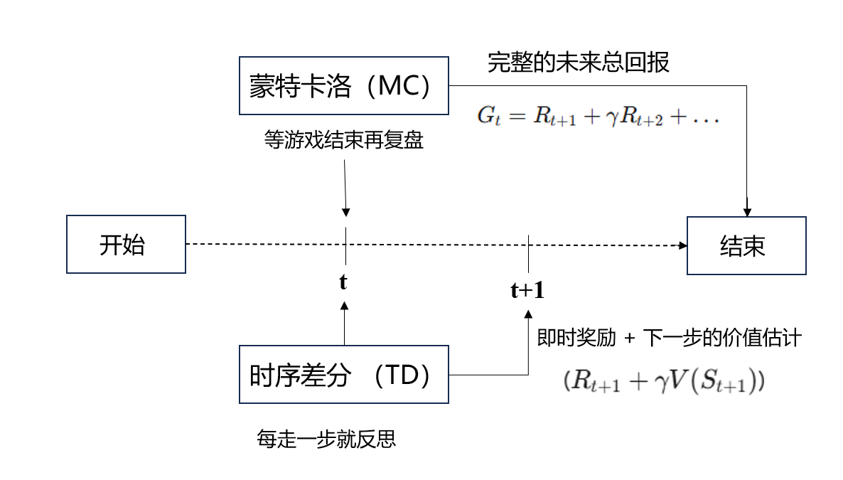
Monte Carlo (MC) methods embody the “post-mortem review” strategy.

They require the agent to wait until a complete episode concludes before updating its estimates. The learning target is the complete, actual cumulative return G_t—the discounted sum of all rewards received from time step t until the end of the episode:

The chief advantage of using G_t as the update target is that it is unbiased.

G_t is a direct, fair sample of the true return based on what actually happened, relying on no intermediate approximations.

However, its drawback is equally significant: high variance.

Because G_t aggregates every source of randomness from time t until the end of the episode, a great early decision might be followed by random missteps later on, resulting in a dismal total return G_t.

This accumulation of uncertainty injects substantial noise into the learning signal, making training unstable and slow to converge.

Temporal Difference Learning (TD)#

Temporal Difference (TD) learning adopts the “reflect on the spot” strategy.

It does not need to wait for an episode to end; in many settings, the agent can learn after every single step.

The core mechanism of TD learning is bootstrapping, inherited from Dynamic Programming: instead of waiting for the full actual return G_t, it constructs a “TD target” by combining the immediate reward r with its current estimate of the next state’s value.

This idea is a cornerstone of modern reinforcement learning and plays a central role in both Value-Based and Actor-Critic architectures.

For example, in Q-Learning, the TD target is used to update Q-values:

In Actor-Critic, it is used to compute the TD error \delta_t that guides the Actor:

where both V(s) and V(s') are estimated by the Critic.

The major advantage of TD learning is low variance.

Because its learning signal (such as \delta_t) depends on the randomness of only a single transition rather than an entire trajectory, training is far more stable and sample-efficient.

The trade-off, however, is that TD targets are biased. Because the TD target relies heavily on an estimate like V(s'), inaccuracies in that estimate—especially early in training—introduce systematic bias into the updates.

Balancing the unbiased, high-variance estimates of Monte Carlo against the biased, low-variance estimates of Temporal Difference (often bridged via techniques like \text{TD}(\lambda) or Generalized Advantage Estimation) remains one of the central design challenges in reinforcement learning.

Trade-offs in Experience Sampling#

As the previous two sections illustrate, when the world model is unknown, finding optimal values shifts from exact computation over a deterministic model (as in Dynamic Programming) to iterative optimization over empirical samples.

Whether in value-based methods like Q-Learning or TD learning more broadly, the core mechanism is continually using new estimates to refine old ones.

This shift has profound implications.

In exact model-based computation, P and R provide an authoritative, noise-free “ground truth.” In sample-based optimization, by contrast, each experience tuple (s,a,r,s') is merely a noisy, partial observation of reality.

Optimization thus becomes a question of how to collect and weight these observations: Which unknown regions of the state-action space should we prioritize exploring to gather informative new samples? And how much weight or trust should we assign to samples generated by different policies or collected at different times?

Reinforcement learning addresses this challenge along three dimensions:

Exploration vs. Exploitation#

First is the balance between Exploration and Exploitation.

To avoid getting trapped in local optima due to limited experience, an agent must constantly choose between executing the best action known so far (exploitation) and trying unfamiliar actions to gather new information (exploration).

Strategies like \epsilon-greedy dynamically adjust the rate of exploration, balancing the need for high-reward trajectories (by exploiting known good actions) against the need for broad state-space coverage (by exploring the unknown).

On-Policy vs. Off-Policy#

On-Policy and Off-Policy methods concern whether the training data matches the agent’s current decision-making policy.

On-Policy methods learn exclusively from data generated by the agent’s current policy, ensuring that feedback directly reflects the policy being optimized. However, this often results in lower sample efficiency, because past experience must be discarded whenever the policy is updated.

Off-Policy methods (such as Q-Learning), by contrast, can learn from historical data or experience collected by entirely different behavior policies. Using techniques like Experience Replay, off-policy algorithms dramatically improve data efficiency, though they must contend with greater training instability when the data distribution diverges from the current policy.

Online Learning vs. Offline Learning#

Online Learning involves learning while actively interacting with the environment in real time (using either the agent’s own exploration strategy or an external behavior policy, such as a random walk), allowing continuous adaptation.

Offline Learning (or Batch RL) attempts to learn an optimal policy purely from a fixed, pre-collected historical dataset, without any further interaction with the environment.

This paradigm is vital for high-stakes real-world domains—such as healthcare or autonomous driving—where live trial-and-error exploration is dangerous or costly, but it places extreme demands on algorithmic generalization and out-of-distribution safety.

By definition, Offline Learning is incompatible with On-Policy updates and therefore relies exclusively on Off-Policy formulations.

Together, these three dimensions govern the sample efficiency, stability, and practical viability of reinforcement learning systems.

Model-Free vs. Model-Based RL#

In reinforcement learning, a “model” refers to anything an agent can use to predict how the environment will respond to its actions—whether an exact analytical specification or a learned approximation.

Model-Free Methods#

Most of the algorithms discussed so far—including Q-Learning, DQN, classic Policy Gradients, and Actor-Critic—fall into the Model-Free category.

These algorithms make no attempt to explicitly learn the environment’s transition dynamics P or reward function R. Instead, they learn a “controller”—either an action-value function Q(s,a) or a policy \pi(a|s)—directly from raw interaction samples (s,a,r,s').

This directly embodies the behaviorist spirit of trial and error: shaping effective behavior patterns purely through repeated action and environmental feedback.

The advantage of model-free methods is that they are relatively straightforward to design and immune to model-approximation errors (since they never build a world model).

The price they pay is low sample efficiency: because the agent cannot simulate or plan ahead in its “imagination,” it typically requires vast amounts of real-world interaction to learn effectively.

Model-Based Methods#

Model-Based methods take the opposite approach, carrying forward the planning spirit of the mathematical/optimal-control tradition.

If an agent can first figure out how the world works, combining that world model with lookahead planning makes decision-making vastly more sample-efficient.

This process typically unfolds in two stages:

1. Model Learning: From interaction experience, the agent learns an approximate model of the environment—estimating transition dynamics \hat{P}(s'|s,a) and rewards \hat{R}(s,a,s') to construct an internal map of the world.
2. Planning: Armed with this (potentially imperfect) internal map \hat{P}, \hat{R}, the agent can simulate future trajectories and plan entirely in its “imagination”—for instance, by running Dynamic Programming updates or Monte Carlo Tree Search (MCTS) to evaluate future possibilities and identify the best action.

The signature strength of model-based RL is exceptional sample efficiency. A single step of real-world interaction can inform thousands of simulated steps inside the agent’s internal world model, dramatically accelerating learning.

Yet this efficiency comes with a major caveat: the learned model \hat{P}, \hat{R} is almost never perfect.

An optimizing RL agent can easily discover and exploit inaccuracies or hallucinations in the learned model, converging on policies that look brilliant in simulation but fail catastrophically in the real world.

Model exploitation and compounding model errors remain the central hurdles for model-based reinforcement learning.

Viewed through this lens, it becomes clear why reinforcement learning has historically shown such a strong affinity for game environments—from early maze navigation and board games to modern video games.

Games sit in a unique “sweet spot” between model-free and model-based paradigms: for most games, the rules are exact, known, and computable, giving us a perfect environment simulator.

This means that even when we use a model-free algorithm, we can run massive parallel simulations to generate virtually limitless, unbiased experience samples (s,a,r,s').

In other words, game environments allow model-free algorithms to enjoy the high practical sample throughput of simulated planning while completely avoiding the model bias and model exploitation risks of learning an approximate world model.

This best-of-both-worlds property has made games the premier proving ground for reinforcement learning.

Many of RL’s most celebrated milestones—such as superhuman performance in Atari, Dota 2, and board games—are testaments to the power of combining model-free learning with massive, perfect simulation.

When Reinforcement Learning Meets Deep Learning#

As we saw in the first two sections, the heart of reinforcement learning lies in iteratively optimizing value functions or policies in an unknown world using empirical samples gathered through interaction.

However, classic tabular methods (such as tabular Q-Learning) hit a fundamental wall when confronted with real-world complexity: the Curse of Dimensionality.

When the state space (such as all possible Go board configurations or raw screen pixels) or action space (such as continuous joint torques on a robot) becomes astronomically large or continuous, storing an exact value for every state-action pair in a table becomes impossible.

To break through this bottleneck, researchers turned to Function Approximation.

Instead of storing an explicit value for every discrete state, we learn a parameterized function with weights \theta—such as Q(s,a;\theta)—to approximate the true values or policy.

The defining power of function approximation is generalization: by extracting salient features of a state s, the model can estimate the value or appropriate action even for states it has never encountered before.

And Deep Neural Networks (DNNs) are the most powerful function approximators known today, capable of automatically learning hierarchical feature representations directly from high-dimensional, raw sensory inputs such as image pixels.

Between 2013 and 2015, marrying reinforcement learning with deep neural networks gave rise to Deep Reinforcement Learning (DRL), vastly expanding the frontier of problems RL could solve.

Deep Value Learning: DQN and the Atari Breakthrough#

The first landmark achievement using deep neural networks as function approximators in RL occurred along the value-based track: DeepMind’s Deep Q-Networks (DQN).

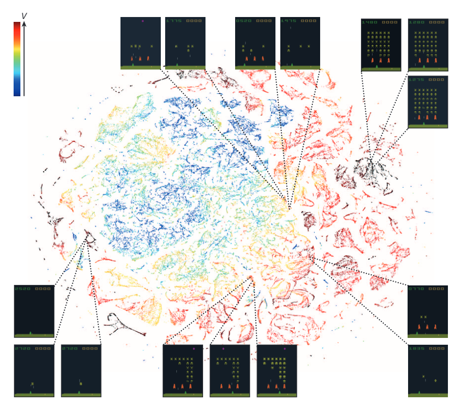
Its goal was simple yet ambitious: enable a single agent to learn how to play a wide variety of Atari 2600 games directly from high-dimensional raw pixel inputs, without any hand-crafted game-specific features.

To achieve this, DQN combined a Convolutional Neural Network (CNN) with classic Q-Learning.

Specifically, it trained a CNN Q(s,a;\theta) that takes raw game frames (state s) as input and outputs the predicted Q-value for every discrete joystick action a.

However, naively combining Q-Learning with nonlinear function approximators like deep neural networks is notoriously prone to training instability and divergence.

DQN overcame this barrier through two critical algorithmic innovations: Experience Replay and a Target Network.

First, Experience Replay breaks the temporal correlation between consecutive training samples.

As the agent plays, it stores transitions (s,a,r,s') in a large replay buffer and trains the network by randomly sampling mini-batches from this pool. This makes the training distribution much closer to independent and identically distributed (i.i.d.), dramatically improving both stability and data efficiency.

Second, the Target Network resolves the “moving target” instability inherent in the Q-Learning update r+\gamma\max_{a'}Q(s',a';\theta).

DQN maintains a separate copy of the network Q(s,a;\theta^-) whose parameters \theta^- are held fixed and only synced with the main network periodically, using it exclusively to compute the TD target:

Holding the target fixed over many gradient steps stabilizes optimization and prevents runaway feedback loops.

Armed with these two innovations, DQN demonstrated for the first time that an agent could learn complex control policies end-to-end from raw sensory inputs, achieving human-level or superhuman performance across dozens of Atari games and ushering in the era of Deep Reinforcement Learning.

AlphaGo: The Synthesis of Learning and Planning#

If DQN demonstrated how deep learning could supercharge model-free value learning, AlphaGo—and its legendary “Move 37”—revealed the immense power of uniting deep reinforcement learning with model-based planning and search.

In 2016, DeepMind’s AlphaGo defeated world Go champion Lee Sedol, marking a historic milestone in which AI surpassed human mastery in the most complex perfect-information board game ever invented.

AlphaGo’s triumph did not rely on a single technique, but on the seamless integration of two core pillars:

1. Deep Learning: Acquiring “Intuition”

• Policy Network \pi(a|s;\theta): A deep CNN trained to predict the most promising next moves, used to narrow and guide the search tree.
• Value Network V(s;\phi): Another deep CNN trained to estimate the win probability from any board position, used to evaluate leaf nodes during search without playing out to the very end.

In the original AlphaGo, these networks were initialized via supervised learning (on human expert games) and refined via reinforcement learning (self-play); its successor, AlphaZero, went a step further by discarding human data entirely and learning purely from tabula rasa self-play.

2. Monte Carlo Tree Search (MCTS): Executing “Planning”

• MCTS is a powerful model-based search and planning algorithm. Leveraging the exact rules of Go (a perfect model of P and R), it performs extensive lookahead simulations in its internal “imagination.”
• The Key Synthesis: During live play, MCTS uses the policy network to prioritize high-probability branches (pruning search breadth) and the value network to evaluate board positions mid-game (pruning search depth).

AlphaGo’s architecture is a masterclass in synthesizing the core trade-offs discussed earlier.

It is fundamentally model-based (relying on MCTS lookahead planning for final move selection), yet it harnesses model-free deep reinforcement learning to train the policy and value networks that act as fast “heuristic intuition”—making lookahead search tractable in Go’s astronomical state space (\sim 10^{170} positions).

At the same time, it takes full advantage of Go as a perfect, deterministic simulation environment.

By wedding deep representation learning (to process complex spatial board states into intuition) with lookahead planning and search (to deliberate over future consequences), AlphaGo established a blueprint for achieving superhuman decision-making.

Together, DQN and AlphaGo revealed the core promise of Deep Reinforcement Learning: combining the perceptual and representational power of deep networks with the sequential decision-making framework of RL to conquer problems with vast state spaces and intricate dynamics.

Frontiers of Reinforcement Learning Applications#

Having traced the intellectual origins of reinforcement learning, dissected its core architectures and trade-offs, and witnessed how deep learning catalyzed the DRL revolution, we now turn to the applied frontier.

Below, we examine how reinforcement learning is driving breakthroughs in two distinct, highly challenging domains: post-training for Large Language Models (LLMs) and Geospatial Artificial Intelligence (GeoAI) for urban planning.

Reinforcement Learning for LLMs#

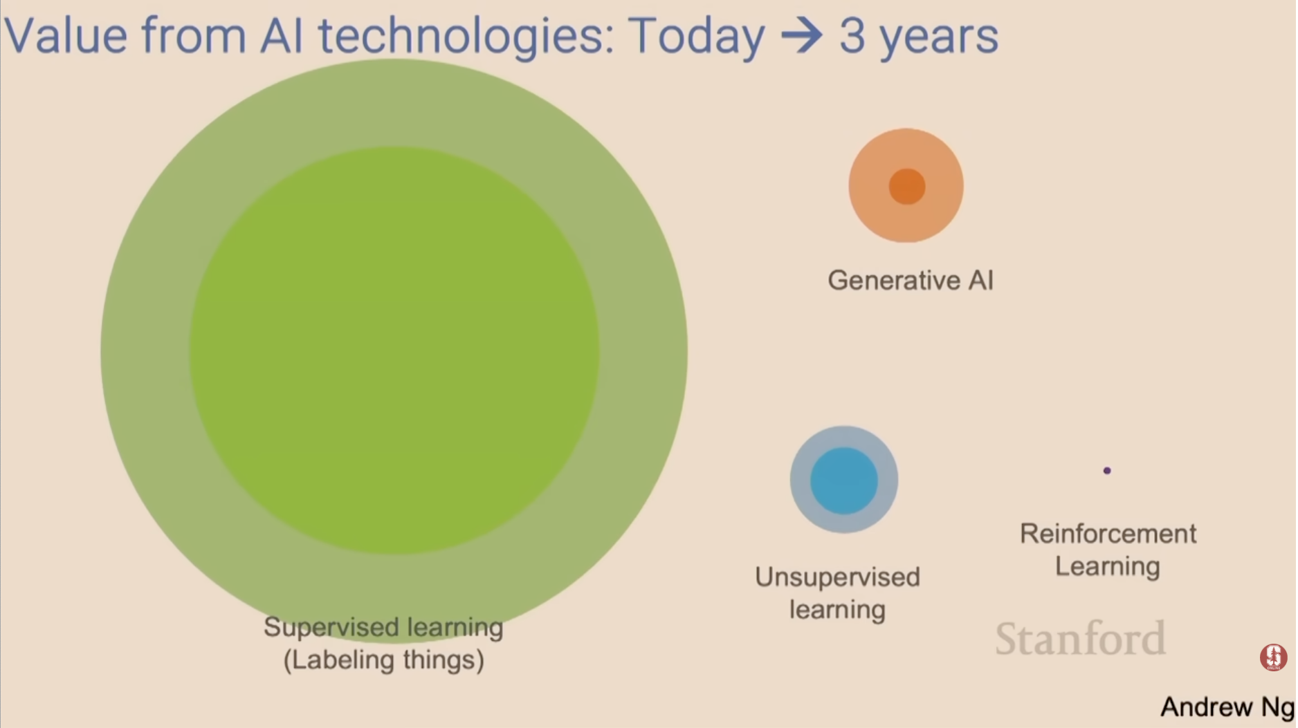
Applying reinforcement learning to the training of Large Language Models has become a defining paradigm for unlocking advanced reasoning capabilities and aligning model behavior with human intent.

This post-training pipeline typically unfolds across several stages.

First is Supervised Fine-Tuning (SFT).

SFT is not reinforcement learning; rather, it is akin to teaching a student how to read instructions and format answers. By training on curated “(instruction, high-quality response)” pairs, a pre-trained LLM learns to follow human instructions and exhibit baseline helpfulness.

Next comes Reinforcement Learning from Human Feedback (RLHF).

Once the model can follow instructions, we want its responses to be more helpful, honest, and harmless.

Standard RLHF trains a separate Reward Model to mimic human preference rankings over candidate responses, and then uses a reinforcement learning algorithm—most commonly Proximal Policy Optimization (PPO)—to fine-tune the LLM to maximize the score assigned by the reward model.

However, traditional PPO-based RLHF faces significant bottlenecks.

PPO requires training and maintaining a separate Value Model (the “Critic”)—typically comparable in size to the LLM itself—to estimate the value of partial text sequences and compute advantage functions.

Because the state space of natural language generation is vast and complex, training an accurate value model is computationally expensive and memory-intensive.

Moreover, relying on a learned neural reward model that imitates human preferences can cap the model’s ceiling, discouraging it from discovering novel reasoning trajectories that surpass human templates.

To overcome these limitations, the DeepSeek team introduced GRPO (Group Relative Policy Optimization) when training their reasoning model DeepSeek-R1.

The core insight of GRPO is to eliminate the expensive Critic (value model) entirely, driving policy updates instead through a streamlined “group competition” mechanism.

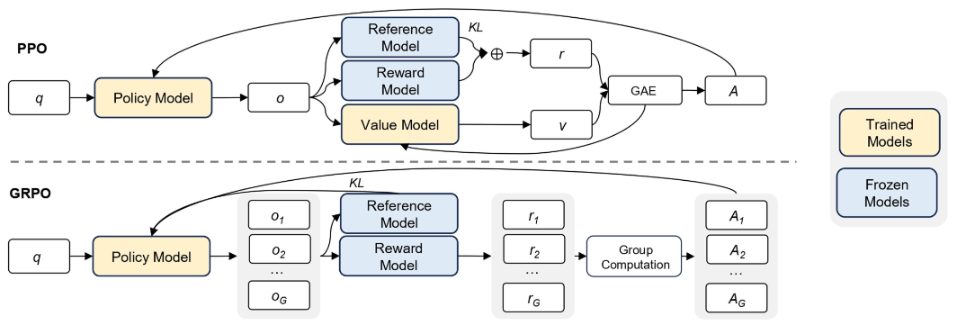
Given a prompt q, GRPO does not ask the LLM to generate just a single response; instead, it samples a group of multiple distinct outputs \{O_1, O_2, \ldots, O_G\}.

Next, an objective “referee”—such as a rule-based answer verifier for math problems or an automated unit-test execution environment for coding tasks—scores each output O_i in the group, assigning an explicit reward r_i.

GRPO’s key innovation lies in recognizing that an effective learning signal does not require knowing the absolute value of a state; rather, it only requires knowing how an answer ranks relative to its peers in the same group.

By normalizing rewards across the sampled group (subtracting the group mean and dividing by the group standard deviation), GRPO directly computes the relative advantage A_i of each response O_i.

Responses that score well above the group average receive a positive advantage A_i and are reinforced; those below average receive a negative advantage and are suppressed.

Through this mechanism of “group sampling, intra-group comparison, and selective reinforcement,” GRPO dramatically simplifies the RL pipeline and eliminates the massive memory and compute overhead of maintaining a separate value network.

In training DeepSeek-R1-Zero, the team went a step further: they bypassed the SFT stage entirely, applying GRPO with rule-based objective rewards directly to the base model. Their hypothesis was that removing human-written reasoning demonstrations would free the model to explore unconstrained, without being tethered to human cognitive habits.

Remarkably, under the pressure of pure, outcome-driven reinforcement learning, DeepSeek-R1-Zero spontaneously developed sophisticated reasoning behaviors—including self-reflection, step-by-step verification, exploring alternative solution paths, and even pausing mid-thought with human-like metacognitive markers such as “Wait, wait. Wait. Let me re-evaluate this step.”

This demonstrates that with the right RL framework and verifiable reward signals, we can incentivize rather than merely imitate deep autonomous reasoning in LLMs.

Of course, raw capabilities emerging from pure RL (“wild growth”) can suffer from poor readability or language mixing.

Consequently, state-of-the-art reasoning LLMs combine pure RL exploration with multi-stage SFT and RLHF alignment, forging agents that pair frontier problem-solving power with human-friendly communication and values.

Applications in GeoAI#

Reinforcement Learning for Urban Planning#

Urban planning—a complex engineering discipline involving high-dimensional spatial configurations, multi-objective trade-offs, and long-term socioeconomic consequences—has traditionally relied heavily on the intuition and experience of human planners.

Confronted with an astronomical combinatorial search space, human designers struggle to manually identify spatial layouts that optimally balance service accessibility, ecological coverage, and construction costs, making the planning workflow time-consuming and suboptimal.

Reinforcement learning (RL), and Deep Reinforcement Learning (DRL) in particular, offers a transformative paradigm by reframing static spatial optimization into a dynamic, sequential decision-making process.

This approach mirrors the iterative workflow of human planners while leveraging computational scale to explore and optimize far beyond human capacity.

1. Sequential Decision-Making and Spatial Layout

Much like a human planner drafting a blueprint step by step, an RL agent constructs a spatial plan incrementally.

In facility location problems, for example, the agent places one new facility at each time step; in land-use allocation, it assigns one functional zone at a time.

This sequential formulation decomposes an intractable, high-dimensional combinatorial optimization problem into a series of manageable single-step decisions, dramatically reducing computational complexity.

2. Dynamic Feedback and Real-Time Adaptation

A city is an interconnected dynamical system where every spatial intervention alters all subsequent possibilities.

RL’s sequential decision framework naturally captures this property. Each time the agent takes an action (e.g., siting a new hospital), the “state” of the urban environment updates immediately (e.g., healthcare coverage in surrounding neighborhoods increases).

This updated spatial state then directly informs the agent’s next decision.

Through this closed-loop feedback mechanism, the planning process accounts for the cascading spatial effects of every action in real time, steering clear of myopic local optima in pursuit of globally coordinated layouts.

3. Flexible, Goal-Oriented Reward Mechanisms

The effectiveness of RL in urban planning rests on its highly adaptable reward structure, characterized by three key properties: delayed evaluation, goal orientation, and multi-objective flexibility.

RL frequently employs delayed rewards—evaluating the comprehensive performance of a spatial layout only after all elements have been placed—which compels the agent to optimize for long-term global outcomes rather than immediate local gains.

Its goal-oriented nature aligns seamlessly with zoning codes and regional planning mandates, allowing planners to encode domain constraints directly into the objective.

Finally, the flexibility of the reward function supports multi-objective optimization: by adjusting reward weights across competing criteria (such as equity, efficiency, and cost), planners can guide the agent to generate diverse Pareto-optimal design alternatives, transforming subjective planning trade-offs into a rigorous, data-driven workflow.

---

While RL’s sequential framework is powerful, a standard RL agent does not natively understand geographic coordinates, polygon geometries, or spatial topology.

To turn RL into a truly data-driven GeoAI tool, we must first solve a foundational representation problem:

How do we translate complex, unstructured urban spatial data into a format that a neural network can read, learn from, and reason over?

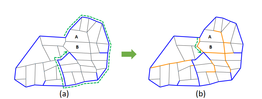
To enable data-driven spatial decision-making, cutting-edge GeoAI research typically abstracts urban space into a Graph structure, where geographic entities (such as demand points, street intersections, or land parcels) form the nodes, and their spatial relationships (such as adjacency, road connectivity, or spatial distance) form the edges.

Once the graph skeleton is constructed, the next step is node feature embedding—injecting domain attributes into each node. These features are carefully divided into two categories to capture both the invariant geography and the evolving state of the city:

• Static Embeddings: Represent invariant node attributes that remain constant throughout the planning episode—most fundamentally, 2D geographic coordinates, alongside baseline demographic or land-use attributes.
• Dynamic Embeddings: The key to intelligent sequential decision-making, these features update in real time after every action taken by the agent. For instance, as new facilities are placed, a node’s “service coverage status” changes; the model tracks this evolution via a dynamic coverage vector, directly informing subsequent placement steps.

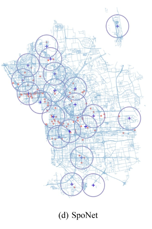
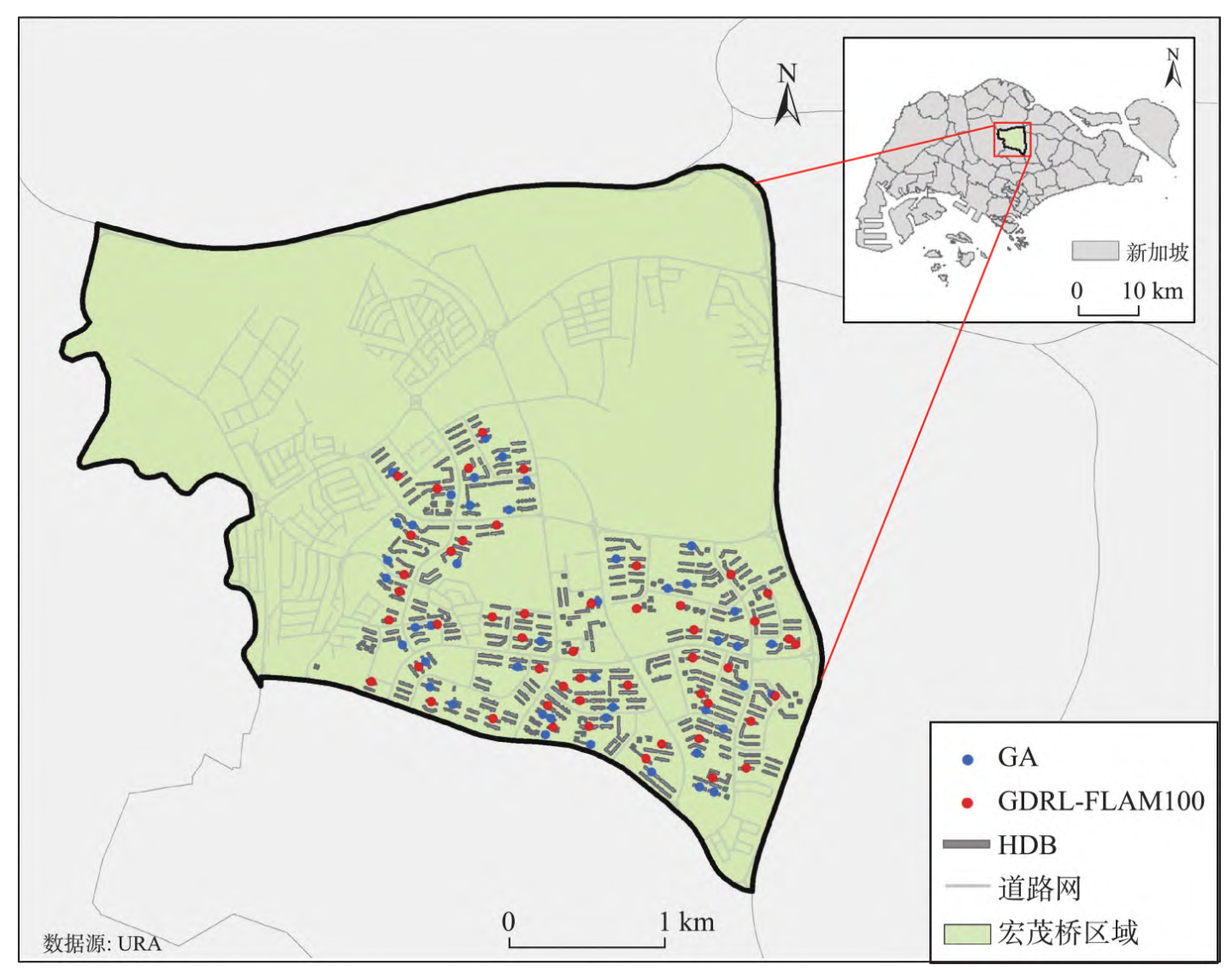
In classic facility location tasks—such as the p-Median problem or the Maximal Covering Location Problem (MCLP)—researchers often represent demand points and candidate facility sites directly as graph nodes.

Here, “demand nodes” correspond to specific geographic locations on the city map that require service coverage, representing the spatial origins of urban demand.

In healthcare facility siting, for example, demand nodes might represent residential communities or apartment blocks, weighted by population to reflect local demand for accessible medical care.

In emergency response planning, demand nodes might represent critical traffic intersections or high-density neighborhoods requiring rapid ambulance or fire-station coverage.

Incorporating rich node weights and socio-spatial attributes allows the RL agent to tailor spatial layouts with high granularity.

RL applied to optimal billboard placement

RL applied to medical station siting

Finally, to enable the model to perceive not just isolated node features but their broader spatial context across the city, researchers pair RL with Graph Neural Networks (GNNs).

Through message passing across graph edges, a GNN allows each node to aggregate feature representations from its spatial neighbors, capturing local neighborhood structure and overall layout efficiency.

Going a step further, recent studies incorporate Graph Attention Networks (GATs), which dynamically compute attention weights across neighboring nodes—allowing the policy network to focus selectively on the nearby locations most critical to the current placement decision.

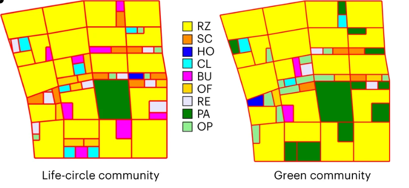
Other Spatial & Urban Applications#

1. Autonomous UAV Path Planning

In complex 3D urban environments, Unmanned Aerial Vehicles (UAVs) must plan trajectories in real time while dodging dynamic obstacles.

Deep reinforcement learning algorithms—such as Deep Deterministic Policy Gradient (DDPG)—enable UAVs to learn flight control policies end-to-end, mapping raw onboard sensor streams (such as LiDAR and camera feeds) directly to flight commands without requiring a pre-built global map.

Through extensive trial-and-error training in physics simulators, UAVs can discover agile navigation strategies—such as hugging building contours in dense urban canyons to minimize travel distance while maintaining safety margins.

These Sim-to-Real workflows are already deployed in industry: for example, NVIDIA uses its Isaac Sim platform alongside reinforcement learning to train autonomous drones for indoor navigation, obstacle avoidance, and automated inventory inspection inside complex warehouses and factories.

2. Cooperative Urban Traffic Signal Control

Traditional fixed-time traffic lights cannot adapt to real-time fluctuations in traffic flow, frequently exacerbating urban congestion. To address this, researchers employ Multi-Agent Deep Reinforcement Learning (e.g., MADDPG), modeling each signalized intersection as an autonomous RL agent.

By processing real-time vehicle queue data captured by intersection cameras, these agents coordinate with neighboring intersections to dynamically adjust green-light phases, optimizing traffic throughput across the entire regional road network.

A prominent real-world deployment of this technology is Hangzhou’s “City Brain” project, developed through a collaboration between Alibaba Group and the Hangzhou municipal government.

By analyzing city-wide traffic flows in real time and dynamically coordinating traffic signals across hundreds of intersections, the system has substantially increased average vehicle speeds in pilot districts and shortened emergency response times for ambulances and fire trucks—demonstrating the tangible impact of reinforcement learning in city-scale infrastructure management.

Epilogue: The Bitter Lesson#

Looking back at the arc of deep learning, we moved from simple, general-purpose MLPs to architectures engineered with strong domain-specific inductive biases—like CNNs for spatial grids and RNNs for sequences—in an effort to “guide” models toward the right representations; yet in the era of the Transformer, the field has swung back toward highly general-purpose architectures scaled with massive compute.

The foundational framework of reinforcement learning—centered on general-purpose learning and search—embodies this exact same spirit of generality.

Does a deeper law underlie this recurring pattern? Should we continue hand-crafting domain-specific inductive biases to guide our agents, or should we place our trust in the scaling power of general-purpose learning mechanisms?

An essay by Richard Sutton offers a provocative answer.

“The Bitter Lesson” is an influential essay published by Richard Sutton on March 13, 2019, on his personal website, Incomplete Ideas.

Its central thesis, drawn from seventy years of AI research history, is unmistakable:

General methods that leverage massive computation ultimately outperform approaches that rely on human domain knowledge—and by a wide margin.

Sutton illustrates this pattern across multiple historical milestones:

• Computer Chess and Go: In chess, the system that finally defeated world champion Garry Kasparov—IBM’s Deep Blue—relied on massive deep search rather than the human-inspired strategic heuristics favored by most AI researchers at the time (a victory that left many human-centric researchers dissatisfied). Twenty years later in Go, AlphaGo—and especially AlphaZero—combined massive compute with self-play reinforcement learning, replacing hand-crafted human Go knowledge with learned intuition and search to achieve superhuman mastery across Go, chess, and shogi alike.
• Speech Recognition and Computer Vision: In 1970s DARPA speech recognition competitions, statistical Hidden Markov Models (HMMs) leveraging computation triumphed over rule-based systems built on human linguistic and acoustic knowledge (such as phonemes and vocal tract modeling). Likewise, in computer vision, early pipelines hand-engineered around edge detection, generalized cylinders, or SIFT features were ultimately swept aside by deep neural networks relying only on general principles like convolution and invariance scaled with compute.

The lesson is “bitter” because it exposes an uncomfortable truth about human vanity in science:

Researchers naturally gravitate toward building their own human understanding and cognitive heuristics into their models. In the short term, injecting domain knowledge yields quick wins and personal satisfaction.

In the long run, however, human-centric heuristics plateau and even become bottlenecks—eventually eclipsed by general-purpose methods that scale effortlessly with Moore’s Law and expanding compute.

Despite our innate preference for human-centric design, Sutton argues that AI researchers must internalize two core takeaways from the Bitter Lesson:

• The Unmatched Power of General-Purpose Methods: We must recognize the supremacy of general methods that continue to scale as computation becomes exponentially cheaper. Across the history of AI, the two foundational methods that scale without bound in this way are search and learning.
• The Irreducible Complexity of the World and Mind: The actual contents of minds and the physical world are “tremendously, irremediably complex.” We should stop trying to hard-code simplified human concepts—about space, objects, or reasoning—into our systems, and instead build meta-methods capable of discovering and capturing arbitrary complexity on their own. Our ultimate goal should be AI agents that discover like we do, not agents pre-loaded with what we have already discovered.

LLMs, Reinforcement Learning, and the Path to AGI#

Are Large Language Models the true path to Artificial General Intelligence (AGI)?

Ever since LLMs began exhibiting striking general-purpose capabilities, debate over this question has raged across the AI community. One camp argues that intelligence is an emergent phenomenon of scale: as we continue scaling model parameters, dataset size, and training compute, higher-order reasoning and general intelligence will naturally emerge—a view seemingly supported by empirical scaling laws.

After all, language is humanity’s primary interface for thought and coordination, and the text of the internet encodes an immense, indirect projection of the physical world, social norms, and human psychology—lending philosophical weight to the idea that “language models the world.”

Yet in a recent podcast interview (consistent with his long-held views), Richard Sutton expressed deep skepticism that the current LLM paradigm can lead to true AGI.

From Sutton’s perspective, standard LLM training fundamentally lacks the direct environmental interaction and experiential grounding required by reinforcement learning: an LLM does not build its own world model from lived experience, but merely learns to imitate humanity’s linguistic descriptions of the world. Because an LLM never directly acts upon the physical world and observes the consequences, it can generate plausible sentences about a boiling kettle without ever truly understanding what it means to touch one.

Proponents of LLMs often counter that pre-trained language models can serve as a rich reservoir of “prior knowledge” to bootstrap subsequent reinforcement learning agents.

Sutton rejects this compromise too, invoking his own Bitter Lesson: methods that rely on human-curated knowledge eventually lose out to general methods that learn directly from experience at scale.

While LLMs certainly consume massive compute, they remain fundamentally tethered to human-generated text and human-summarized knowledge. In Sutton’s view, building on human imitation is starting on the wrong foundation.

appearing later on the very same podcast series, Andrej Karpathy (former Director of AI at Tesla and a founding member of OpenAI) offered a compelling, pragmatic counterpoint.

Karpathy acknowledged that “The Bitter Lesson” has become near-scripture in modern AI labs, with researchers constantly asking whether their methods align with compute-driven generality rather than human cognitive biases.

However, he characterized Sutton’s purist stance—Learning from scratch purely through environmental interaction—as “classical” and overly idealized when applied to the messy reality of building general intelligence.

While it is true that AlphaZero (trained with zero human data) decisively outperformed AlphaGo (initialized with human games)—a textbook validation of the Bitter Lesson—Karpathy pointed out that board games with closed, compact rules are a far cry from the open-ended complexity of the real world.

To illustrate, Karpathy used the analogy of a newborn zebra: within minutes of birth, a zebra foal can stand up and run alongside its mother. That intricate sensorimotor capability is not learned from scratch via reinforcement learning during the foal’s lifetime—if a newborn zebra had to learn locomotion from random muscle twitches via trial and error, it would be eaten by a lion on day one. Instead, that baseline competence is hard-wired by billions of years of biological evolution.

Taking a pragmatic engineering view, Karpathy likened LLM pre-training on internet text to a “crappy version of evolution.”

Because humans do not have access to the planetary-scale evolutionary simulator that shaped animal brains, pre-training on the collective corpus of human knowledge serves as an indispensable cold-start prior—initializing the neural network with rich representations before reinforcement learning takes over to refine reasoning and agency. Indeed, this hybrid recipe (Pre-training + RL post-training) is precisely how today’s frontier AI labs operate.

In Karpathy’s view, while LLMs still lack many of the grounded, continual-learning capabilities of biological animals—and while Sutton’s Bitter Lesson remains a north star—treating internet pre-training as an evolutionary warm start is the most practical path forward today.

Authors & References#

This chapter was authored by Guolong Li, Zhixiong Xiao, and Binghan Li with assistance from AI tools. Several illustrations used in the text are adapted from public online sources.

The cover illustration was generated using Jimeng AI (即梦 AI) with the following prompt:

In a futuristic world composed of swirling nebulae and flowing data streams, a robot explores the core of learning. Floating around it are multiple translucent scrolls, each displaying a classic maze or treasure map, symbolizing the processes of exploration and decision-making in reinforcement learning. On several scrolls, the explored paths end in dead ends, glowing red to represent failure; on the scroll held high by the robot, a complete pathway is illuminated in golden light, symbolizing its discovery of the optimal solution after无数 trials and errors. Nearby, a companion robot quietly observes with a glowing ancient book open before it, as if comparing theoretical book knowledge against the learner’s lived empirical experience.

References#

1. The Bitter Lesson — Richard Sutton (2019)

2. Andrew Ng: Opportunities in AI (2023)

3. Dwarkesh Podcast: Richard Sutton — Father of RL thinks LLMs are a dead end

4. Dwarkesh Podcast: Andrej Karpathy — “We’re summoning ghosts, not building animals”

5. Sutton, R. S., & Barto, A. G. (1998). Reinforcement learning: An introduction (Vol. 1). MIT Press, Cambridge.

6. Guo, D., Yang, D., Zhang, H., Song, J., Wang, P., Zhu, Q., Xu, R., Zhang, R., Ma, S., & Bi, X. (2025). DeepSeek-R1 incentivizes reasoning in LLMs through reinforcement learning. Nature, 645(8081), 633–638.

7. Mnih, V., Kavukcuoglu, K., Silver, D., Graves, A., Antonoglou, I., Wierstra, D., & Riedmiller, M. (2013). Playing Atari with deep reinforcement learning. arXiv preprint arXiv:1312.5602.

8. Mnih, V., Kavukcuoglu, K., Silver, D., Rusu, A. A., Veness, J., Bellemare, M. G., Graves, A., Riedmiller, M., Fidjeland, A. K., & Ostrovski, G. (2015). Human-level control through deep reinforcement learning. Nature, 518(7540), 529–533.

9. Zheng, Y., Lin, Y., Zhao, L., Wu, T., Jin, D., & Li, Y. (2023). Spatial planning of urban communities via deep reinforcement learning. Nature Computational Science, 3(9), 748–762.

10. Lai, X., Yang, Z., Xie, J., & Liu, Y. (2024). Reinforcement learning in transportation research: Frontiers and future directions. Multimodal Transportation, 3(4), 100164.

11. Zheng, Y., Su, H., Ding, J., Jin, D., & Li, Y. (2023, August). Road planning for slums via deep reinforcement learning. In Proceedings of the 29th ACM SIGKDD Conference on Knowledge Discovery and Data Mining (pp. 5695–5706).

12. Liang, H., Wang, S., Li, H., Zhou, L., Chen, H., Zhang, X., & Chen, X. (2024). Sponet: Solve spatial optimization problem using deep reinforcement learning for urban spatial decision analysis. International Journal of Digital Earth, 17(1), 2299211.

13. Zhong, Y., Wang, S., Liang, H., Wang, Z., Zhang, X., Chen, X., & Su, C. (2024). ReCovNet: Reinforcement learning with covering information for solving maximal coverage billboards location problem. International Journal of Applied Earth Observation and Geoinformation, 128, 103710.

14. Sutton, R. S., & Barto, A. G. (2018). Reinforcement learning: An introduction (2nd ed.). MIT Press.

15. Arulkumaran, K., Deisenroth, M. P., Brundage, M., & Bharath, A. A. (2017). Deep reinforcement learning: A brief survey. IEEE Signal Processing Magazine, 34(6), 26–38.

16. Wang, Z., & Cao, K. (2024). Intelligent site selection method for public service facilities coupling improved graph attention network and deep reinforcement learning (耦合改进图注意力网络与深度强化学习的公共服务设施智能化选址方法). Journal of Geo-information Science (地球信息科学学报), 26(11), 2452.